When you create a histogram with statistical software, the software uses the data (including the sample size) to automatically choose the width and location of the histogram bins. The resulting histogram is an attempt to balance statistical considerations, such as estimating the underlying density, and "human considerations," such as choosing "round numbers" for the location and width of bins for histograms. Common "round" bin widths include 1, 2, 2.5, and 5, as well as these numbers multiplied by a power of 10.
The default bin width and locations tend to work well for 95% of the data that I plot, but sometimes I decide to override the default choices. This article describes how to set the width and location of bins in histograms that are created by the UNIVARIATE and SGPLOT procedures in SAS.
Why override the default bin locations?
The most common reason to override the default bin locations is because the data have special properties. For example, sometimes the data are measured in units for which the common "round numbers" are not optimal:
- For a histogram of time measured in minutes, a bin width of 60 is a better choice than a width of 50. Bin widths of 15 and 30 are also useful.
- For a histogram of time measured in hours, 6, 12, and 24 are good bin widths.
- For days, a bin width of 7 is a good choice.
- For a histogram of age (or other values that are rounded to integers), the bins should align with integers.
You might also want to override the default bin locations when you know that the data come from a bounded distribution. If you are plotting a positive quantity, you might want to force the histogram to use 0 as the leftmost endpoint. If you are plotting percentages, you might want to force the histogram to choose 100 as the rightmost endpoint.
To illustrate these situations, let's manufacture some data with special properties. The following DATA step creates two variables. The T variable represents time measured in minutes. The program generates times that are normally distributed with a mean of 120 minutes, then rounds these times to the nearest five-minute mark. The U variable represents a proportion between 0 and 1; it is uniformly distributed and rounded to two decimal places.
data Hist(drop=i); label T = "Time (minutes)" U = "Uniform"; call streaminit(1); do i = 1 to 100; T = rand("Normal", 120, 30); /* normal with mean 120 */ T = round(T, 5); /* round to nearest five-minute mark */ U = rand("Uniform"); /* uniform on (0,1) */ U = floor(100*U) / 100; /* round down to nearest 0.01 */ output; end; run; |
How do we control the location of histogram bins in SAS? Read on!
Custom bins with PROC UNIVARIATE: An example of a time variable
I create histograms with PROC UNIVARIATE when I am interested in also computing descriptive statistics such as means and quantiles, or when I want to fit a parametric distribution to the data. The following statements create the default histogram for the time variable, T:
title "Time Data (N=100)"; ods select histogram(PERSIST); /* show ONLY the histogram until further notice */ proc univariate data=Hist; histogram T / odstitle=title odstitle2="Default Bins"; run; |
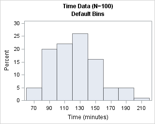
The default bin width is 20 minutes, which is not horrible, but not as convenient as 15 or 30 minutes. The first bin is centered at 70 minutes; a better choice would be 60 minutes.
The HISTOGRAM statement in PROC UNIVARIATE supports two options for specifying the locations of bins. The ENDPOINTS= option specifies the endpoints of the bins; the MIDPOINTS= option specifies the midpoints of the bins. The following statements use these options to create two customize histograms for which the bin widths are 30 minutes:
proc univariate data=Hist; histogram T / midpoints=(60 to 210 by 30) odstitle=title odstitle2="Midpoints"; run; proc univariate data=Hist; histogram T / endpoints=(60 to 210 by 30) odstitle=title odstitle2="Endpoints"; run; |
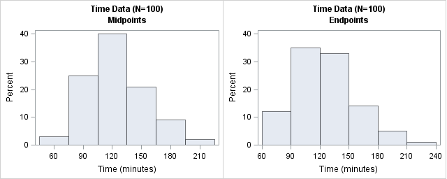
The histogram on the left has bins that are centered at 30-minute intervals. This histogram makes it easy to estimate that about 40 observations are approximately 120 minutes. The counts for other half-hour increments are similarly easy to estimate. In contrast, the histogram on the right has bins whose endpoints are 60, 90, 120,... minutes. With this histogram, it easy to see that about 35 observations have times that are between 90 and 120 minutes. Similarly, you can estimate the number of observations that are greater than three hours or less than 90 minutes.
Both histograms are equally correct. The one you choose should depend on the questions that you want to ask about the data. Use midpoints if you want to know how many observations have a value; use endpoints if you want to know how many observations are between two values.
If you run the SAS statements that create the histogram on the right, you will see the warning message
WARNING: The ENDPOINTS= list was extended to accommodate the data.
This message informs you that you specified the last endpoint as 210, but that additional bins were created to display all of the data.
Custom bins for a bounded variable
As mentioned earlier, if you know that values are constrained within some interval, you might want to choose histogram bins that incorporate that knowledge. The U variable has values that are in the interval [0,1), but of course PROC UNIVARIATE does not know that. The following statement create a histogram of the U variable with the default bin locations:
title "Bounded Data (N=100)"; proc univariate data=Hist; histogram U / odstitle=title odstitle2="Default Bins"; run; |
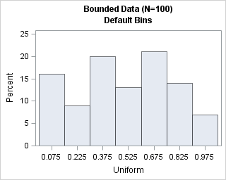
The default histogram shows seven bins with a bin width of 0.15. From a statistical point of view, this is an adequate histogram. The histogram indicates that the data are uniformly distributed and, although it is not obvious, the left endpoint of the first bin is at 0. However, from a "human readable" perspective, this histogram can be improved. The following statements use the MIDPOINTS= and ENDPOINTS= options to create histograms that have bin widths of 0.2 units:
proc univariate data=Hist; histogram U / midpoints=(0 to 1 by 0.2) odstitle=title odstitle2="Midpoints"; run; proc univariate data=Hist; histogram U / endpoints=(0 to 1 by 0.2) odstitle=title odstitle2="Endpoints"; run; ods select all; /* turn off PERSIST; restore normal output */ |
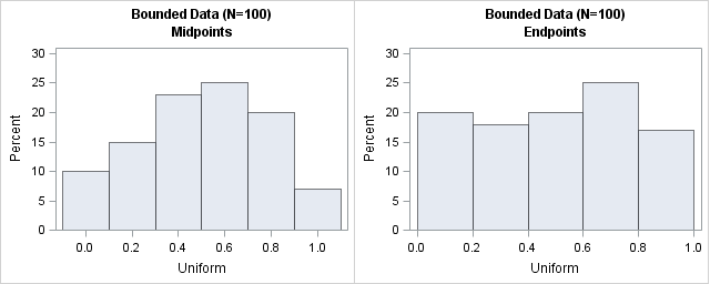
The histogram on the left is not optimal for these data. Because we created uniformly distributed data in [0,1], we know that the expected count in the leftmost bin (which is centered at 0) is half the expected count of an inner bin. Similarly, the expected count in the rightmost bin (which is centered at 1) is half the count of an inner bins because no value can exceed 1. Consequently, this choice of midpoints is not very good. For these data, the histogram on the right is better at revealing that the data are uniformly distributed and are within the interval [0,1).
Custom bins with PROC SGPLOT
If you do not need the statistical power of the UNIVARIATE procedure, you might choose to create histograms with PROC SGPLOT. The SGPLOT procedure supports the BINWIDTH= and BINSTART= options on the HISTOGRAM statement. The BINWIDTH= option specifies the width for the bins. The BINSTART= option specifies the center of the first bin.
I recommend that you specify both the BINWIDTH= and BINSTART= options, and that you choose the bin width first. Be aware that not all specifications result a valid histogram. If you make a mistake when specifying the bins, you might get the following error
WARNING: The specified BINWIDTH= value will be ignored in order to accommodate the data.
That message usually means that the minimum value of the data was not contained in a bin.
For a bin width of h, the BINSTART= value must be less than xmin + h/2, where xmin is the minimum value of the data.
By default, the axis does not show a tick mark for every bin, but you can force that behavior by using the SHOWBINS option. The following statements call the SGPLOT procedure to create histograms for the time-like variable, T. The results are again similar to the custom histograms that are shown in the previous section:
title "Time Data (N=100)"; title2 "Midpoints"; proc sgplot data=Hist; histogram T / binwidth=15 binstart=60 showbins; /* center first bin at 60 */ run; title2 "Endpoints"; proc sgplot data=Hist; histogram T / binwidth=15 binstart=52.5; /* 52.5 = 45 + h/2 */ xaxis values=(45 to 180 by 15); /* alternative way to place ticks */ run; |
The following statements call the SGPLOT procedure to create histograms for the bounded variable, U. The results are similar to those created by the UNIVARIATE procedure:
title "Bounded Data (N=100)"; title2 "Midpoints"; proc sgplot data=Hist; histogram U / binwidth=0.2 binstart=0 showbins; /* center first bin at 0 */ run; title2 "Endpoints"; proc sgplot data=Hist; histogram U / binwidth=0.2 binstart=0.1; /* center first bin at h/2 */ xaxis values=(0 to 1 by 0.2); run; |
In summary, for most data the default bin width and location result in a histogram that is both statistically useful and easy to read. However, the default choices can lead to a less-than-optimal visualization if the data have special properties, such as being time intervals or being bounded. In those cases, it makes sense to choose a bin width and a location of the first bin such that reveals your data's special properties. For the UNIVARIATE procedure, use the MIDPOINTS= or ENDPOINTS= options on the HISTOGRAM statement. For the SGPLOT procedure, use the BINWIDTH= and BINSTART= options to create a histogram with custom bins.

5 Comments
Pingback: Comparative histograms: Panel and overlay histograms in SAS - The DO Loop
Thanks for this. I was trying to use SGPLOT histogram with BINSTART for the first time. Until reading this post, I didn't realize that you need to specify the *center* for first bin rather than the *start* of the first bin.
i have question regarding proc template to create histogram where i can control the x axis interval lets say of 5.
code i was working on is this one
proc template;
define statgraph temp;
begingraph;
entrytitle " ";
layout lattice / columns=2 columngutter=5px
columndatarange=data
rowdatarange=unionall ;
histogram var/ binaxis=false;
endlayout;
endgraph;
end;
run;
proc sgrender data=test_stat1 template=Absbiases;
by product SensorLotNumber;
dynamic var="var";
run;
You can ask programming questions at the SAS Support Communities. Here is a link to the documentation for the HISTOGRAM statement, which shows the syntax for creating a histogram and the syntax for the BINSTART= and BINWIDTH= options.
Pingback: Create filled density plots in SAS - The DO Loop