While at SAS Global Forum 2014 I attended a talk by Jorge G. Morel on the analysis of data with overdispersion. (His slides are available, along with a video of his presentation.) The Wikipedia defines overdispersion as "greater variability than expected from a simple model." For count data, the "simple model" is the Poisson model, for which the variance equals the mean. Morel pointed out that the variance of count data is often greater than is permitted under a Poisson model, so more complicated models must be used.
One model that is used is the negative binomial model, for which the variance is greater than the mean. One of Morel's slides (Slide 43) mentions that the Poisson and NB distributions are closely related: you can view the negative binomial as a Poisson(λ) distribution, where λ is a gamma-distributed random variable. A distribution that has a random parameter is called a compound distribution.
In school I learned that the negative binomial is the distribution of the number of failures before k successes in a sequence of independent Bernoulli trials, which doesn't seem to be related to a Poisson distribution. To better understand Morel's talk, I wrote a SAS/IML program that simulates a random variable drawn from a Poisson(λ) distribution, where λ is drawn from a gamma distribution. The program shows off a feature of SAS/IML 12.1, namely that you can pass vectors of parameters as arguments to the RANDGEN subroutine. Here is the program:
/* Simulate X from a compound distribution: X ~ Poisson(lambda), where lambda ~ gamma(a,b). Parameters from Morel's talk at SASGF14. E(X) = mu = a*b = 10; Var(X) = mu*(1+mu/a) which is greater than mu */ proc iml; N = 1000; a = 5; b = 2; call randseed(12345); lambda = j(N,1); call randgen(lambda, "Gamma", a, b); /* lambda ~ Gamma(a,b) */ x = j(N,1); call randgen(x, "Poisson", lambda); /* 12.1 feature: pass vector of parameters */ |
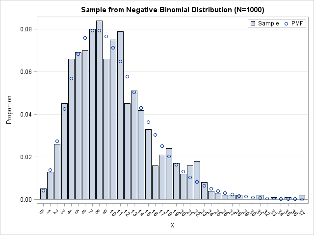
The distribution of these simulated data agrees with the theoretical NB distribution (Slide 44 of Morel's presentation). In the following graph, the bar chart is the empirical distribution of the simulated data, whereas the circles represent the NB probability density. The graph was created by using the techniques in Chapter 3 of my book Simulating Data with SAS.
Upon doing further reading I learned that the compound distribution definition of the NB is favored by the insurance industry. Each policy holder has a different risk of getting in an accident, so the rate of claims (the λ parameter) is treated as random. The gamma distribution is a flexible way to model the distribution of risks in the population.
Of course, SAS enables you to sample directly from the negative binomial distribution, but that requires the traditional parameterization in terms of failures and the probability of success in a Bernoulli trial. This formulation in terms of a compound distribution enables you to use parameters that are more interpretable in certain applications.


2 Comments
Hi Rick--
Another angle on how closely the two are related is shown in our entry http://sas-and-r.blogspot.com/2011/03/example-830-compare-poisson-and.html, where I demonstrate that the cumulative probabilities for the negative binomial approach those from the Poisson, as the size increases.
I now default to using negative binomial models for all count outcomes, as it seems the cost (1 additional DF) is small and the benefit of the additional flexibility is great.
Pingback: Convenient functions vs. efficient subroutines: Your choice - The DO Loop