
This article describes how to generate random samples from the multinomial distribution in SAS. The content is taken from Chapter 8 of my book Simulating Data with SAS.
The multinomial distribution is a discrete multivariate distribution. Suppose there are k different types of items in a box, such as a box of marbles with k different colors. Let pi be the probability of drawing an item of type i, where Σi pi = 1. If you draw N items with replacement, you will obtain N1 items of the first type, N2 items of the second type, and so forth, where Σi Ni = N. The k-tuple of counts (N1, N2, ..., Nk) is a single draw from the multinomial distribution.
For example, suppose you want to draw socks (with replacement) from a big box that contains socks of k = 3 different colors. After each draw, you record the color of the sock, replace it in the box, and mix the contents well so that the probabilities of drawing each color are unchanged. If you draw N = 100 socks, you might get 48 black socks, 21 brown socks, and 31 white socks. That triplet of values, (48, 21, 31), is a single observation for the multinomial distribution of three categories (the colors). Of course, repeating the experiment will, in general, result is a different triplet of counts. The distribution of those counts is the multinomial distribution. The scatter plot at the top of this article visualizes the distribution for the parameters p = (0.5, 0.2, 0.3) and for N = 100. Notice that only two counts are shown; the third count is 100 minus the sum of the first two counts.
Notice that if there are only two categories with selection probabilities, p and 1 – p, then the multinomial distribution is equivalent to the binomial distribution with parameter p in the sense that the count N1 is binomially distributed (and so is N2).
You can sample from the multinomial distribution in SAS by using the RANDMULTINOMIAL function in SAS/IML software. The syntax of the RANDMULTINOMIAL function is
X = RandMultinomial(SampleSize, NumTrials, Prob); |
The following statements generate a 1000 x 3 matrix, where each row is a random observation from a multinomial distribution. The probability of drawing a black sock is 0.5. The probability of drawing a brown sock is 0.2. The probability of drawing a white sock is 0.3.
proc iml;
call randseed(4321);                   /* set random number seed */
c = {"black", "brown", "white"};
prob = {0.5     0.2       0.3};        /* probabilities of pulling each color */
X = RandMultinomial(1000, 100, prob);  /* 1000 draws of 100 socks with 3 colors */
print X[colname=c]; |
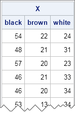
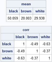
Each row shows the frequencies that result from drawing 100 socks (with replacement). Consequently, the sum of each row is 100. Although there is variation within each column, elements in the first column are usually close to the expected value of 50, elements in the second column are close to 20, and elements in the third column are close to 30. You can see this by computing the column means. You can also compute the correlation matrix, which shows that the variables are negatively correlated with each other. This makes sense: There are exactly 100 items in each draw, so if you draw more of one color, you will have fewer of the other colors.
mean = mean(X);
corr = corr(X);
print mean[colname=c],
corr[colname=c rowname=c format=BEST5.]; |
You can visualize the multinomial distribution by plotting the first two components against each other, as shown at the beginning of this post. The multinomial distribution is a discrete distribution whose values are counts, so there is considerable overplotting in a scatter plot of the counts. One way to resolve the overplotting is to overlay a kernel density estimate. Areas of high density correspond to areas where there are many overlapping points.
create MN from X[c=c]; append from X; close MN; quit; ods graphics on; proc kde data=MN; bivar black brown / bwm=1.5 plots=ContourScatter; run; |
The density overlay shows that most of the density is near the population mean (50, 20). The scatter plot overlay shows the negative correlation in the simulated data, and also that some observations are far from the mean.
If you don't have SAS/IML software, you can still simulate multinomial data by using the "table distribution" in the data step. There is also a clever way to use PROC SURVEYSELECT to generate multinomial data. My next blog post presents those alternate computations.

4 Comments
Pingback: Alternate ways to simulate multinomial data - The DO Loop
Pingback: Balls and urns Part 2: Multi-colored balls - The DO Loop
Pingback: Sample with replacement and unequal probability in SAS - The DO Loop
Pingback: Simulate from the multinomial distribution in the SAS DATA step - The DO Loop