This article describes how to implement the truncated normal distribution in SAS. Although the implementation in this article uses the SAS/IML language, you can also implement the ideas and formulas by using the DATA step and PROC FCMP. For reference, I recommend the Wikipedia article on the truncated normal distribution.
The truncated normal distribution contains two parts: a normal distribution N(μ, σ), and an interval of truncation [a, b]. Denote the four-parameter truncated normal distribution by TN(μ, σ, a, b). There are four essential functions that you need when you are working with a statistical distribution. You need to know how to generate random values, how to compute the density (PDF), how to compute the cumulative distribution (CDF), and how to compute quantiles (inverse CDF).
The example in this article specifies a finite interval, which results in doubly-truncated distribution. However, the functions are written to support a one-sided truncation. To generate a distribution that is truncated on the right, specify a = .M so that the truncation interval is (–∞, b]. To generate a distribution that is truncated on the left, specify b = .P so that the truncation interval is [a, ∞).
Random values of the truncated normal distribution
There are two ways to generate random values. The most intuitive method is an acceptance-rejection algorithm: simulate X ~ N(μ, σ) and then reject and discard any values that are outside the interval [a, b]. That technique works well when the probability that X is in the interval [a, b] is reasonably large, but there are general issues that you have to overcome when you implement an acceptance-rejection algorithm in a vector language.
The inverse CDF method for random number generation is easier to implement. If F is the (cumulative) distribution function, then the following steps generate a random variate for the truncated distribution on [a, b]:
- Generate a uniform random value u in the interval [F(a), F(b)].
- Compute the quantile (inverse CDF) for u. That is, compute x = F–1(u).
proc iml;
/* Random sample from TN on [a,b] by using inverse CDF method */
start randTN(N, mu, sigma, a, b);
   /* Support one-sided truncation. Define Phi(.M)=0 and Phi(.P)=1 */
   cdf_a = choose(a=., 0, cdf("Normal", a, mu, sigma));  /* Phi(a) */
   cdf_b = choose(b=., 1, cdf("Normal", b, mu, sigma));  /* Phi(b) */
   u = j(N,1,.);
   call randgen(u, "Uniform");           /* U ~ U(0,1) */
   z = cdf_a + (cdf_b - cdf_a)*u;        /* Z ~ U(Phi(a), Phi(b)) */
   x = quantile("Normal", z, mu, sigma); /* x always in [a,b] */
   return(x);
finish;

/* test: generate 1,000 random values from the truncated normal */
call randseed(12345);
mu = 1; sigma = 0.8;  a = 0;  b = 3;     /* parameters of the distribution */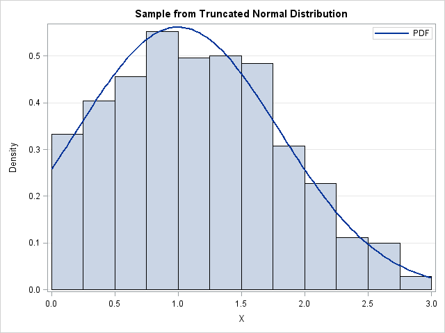
x = randTN(1000, mu, sigma, a, b); |
A histogram of the random sample is shown at the top of this post. The histogram is overlaid with a curve that shows the PDF for the truncated normal distribution, which is computed in the next section.
The PDF for the truncated normal distribution
Computing the density function for the truncated normal distribution is easy. You simply use the usual normal PDF on [a, b], but scale the density function so that it integrates to one:
start pdfTN(x, mu, sigma, a, b);
   /* Support one-sided truncation. Define Phi(.M)=0 and Phi(.P)=1 */
   cdf_a = choose(a=., 0, cdf("Normal", a, mu, sigma));  /* Phi(a) */
   cdf_b = choose(b=., 1, cdf("Normal", b, mu, sigma));  /* Phi(b) */
   return( pdf("Normal", x, mu, sigma) / (cdf_b - cdf_a) );
finish;

/* test: generate PDF on [a, b] */
t = do(a, b, (b-a)/100);
y = pdfTN(t, mu, sigma, a, b); |
The CDF for the truncated normal distribution
You can express the CDF for the truncated normal distribution in terms of the CDF for the normal distribution. You just need to translate and scale the normal CDF appropriately:
start cdfTN(x, mu, sigma, a, b);
   /* Support one-sided truncation. Define Phi(.M)=0 and Phi(.P)=1 */
   cdf_a = choose(a=., 0, cdf("Normal", a, mu, sigma));  /* Phi(a) */
   cdf_b = choose(b=., 1, cdf("Normal", b, mu, sigma));  /* Phi(b) */
   y = (cdf("Normal", x, mu, sigma) - cdf_a)/ (cdf_b - cdf_a);
   /* If x < a, return 0. If x > b, return 1. */
   if a^=. then do;
      idx = loc(x < a); if ncol(idx)>0 then y[idx] = 0;
   end;
   if b^=. then do;
      idx = loc(x > b); if ncol(idx)>0 then y[idx] = 1;
   end;
   return( y );
finish;

/* test: generate CDF on [a, b] */
t = do(a, b, (b-a)/100);
cdf = cdfTN(t, mu, sigma, a, b); |
Quantiles for the truncated normal distribution
Once again, it is easy to compute quantiles of the truncated normal in terms of quantiles of the normal distribution. You just have to scale the normal CDF function appropriately:
start QuantileTN(p, mu, sigma, a, b);
   /* Support one-sided truncation. Define Phi(.M)=0 and Phi(.P)=1 */
   cdf_a = choose(a=., 0, cdf("Normal", a, mu, sigma));  /* Phi(a) */
   cdf_b = choose(b=., 1, cdf("Normal", b, mu, sigma));  /* Phi(b) */
   return( quantile("Normal", cdf_a + (cdf_b - cdf_a)*p, mu, sigma) );
finish;

q = quantileTN(y, mu, sigma, a, b); |
Conclusions
The PDF, CDF, QUANTILE, and RAND functions in SAS support distributions that arise often in practice. As shown in this article, you can use these basic distributions as building blocks to define new distributions, such as the truncated normal distribution or the folded normal distribution.
Truncated normal distributions arise in various regression models, such as regression models for the heights of soldiers in the military because there are often height limits for recruits. You can also use the truncated normal distribution to model student scores on standardized tests such as the SAT, for which 200 is the lowest possible score on each test.

13 Comments
Pingback: How to choose parameters so that a distribution has a specified mean and variance - The DO Loop
The CDF idea is brilliant. What if I want to generate a multivariate normal distribution? For example,
proc iml;
a=randnormal(100,0,1); *Actually a standard normal distribution;
b=randnormal(30,a,I(100)); *Generate a multivariate normal dist from a;
quit;
For the dist b, I would like to truncate b within the interval [-3,3]. I can write a do loop and if then statement to achieve that goal. In CDF call routines, I don't know if there is a multivariate normal distribution.
Thanks for your time!
Multivariate normal distributions have CDFs (I've written about the 2D bivariate normal) but you can't use it as you describe. There are many points that all have the same CDF value. In 2D the inverse image (quantile) of a probability value is a curve, in 3D it is a surface, etc.
You can use the acceptance-rejection technique. I don't know any other nifty tricks, but I hope you will research the problem and report back if you find something.
Rick or viewers, I am new to IML and have not been able to write a code to implement a truncated multivariate normal distribution. I am trying to generate a sample of multivariate correlated data truncated below at 0 and above at 1. For instance, if I wanted to simulate a distribution of "probabilities of an event", then the resulting PDs would need to be truncated over the (0,1) interval. Can anyone provide any guidance? (By the way, thanks to my purchase of Rick's Simulating Data with SAS, I can produce univariate results that are truncated over the interval, but I cannot extend it to multivariate without some additional guidance. Thank you!
I should also mention that I am trying to generate 10,000 random draws, so I generated 25,000 and then simply excluded the draws outside of my desired interval. I have 19 variables, so I created a 25,000 x 19 matrix with each columns reflecting the marginal distribution for the corresponding variable.
I think I read somewhere (perhaps in Dr. Wicklin's text) that this approach could cause bias in the results.
So, I examined the marginal distributions for the individual columns in my output and I found that they do not appear to be normally distributed....nor do theie means and standard deviations match what I previously prescribed....this doesn't seem totally surprising to me. Should a truncated multivariate normal distribution retain the marginal distributions' characteristics? Further, should it retain the prescribed correlation structure that was imposed prior to excluding the results the existed outside of the chosen interval? I expect not.....So, let's assume I have 3 variables, each with a mean of 0.50 and a standard deviation of 0.75 and each with a pair wise correlation of 0.30. How do I simulate a truncated multivariate distribution with these characteristics so that resulting random variates are limited to the interval (0,1) and that correlation structure is retained? It doesn't seem reasonable to me to think that the standard deviation could be retained with the interval restriction. Am I missing something? Thanks!
Discussions of this type are more easily conducted at the SAS Support Communities. To answer your questions: When you truncate data, the marginal distributions and the covariance structure will no longer match what you originally specified. As you say, the variances and covariances must change when you restrict the data to a smaller range.
Thanks. I will move over to the SAS Support Communities - thanks again!
Brian
Sounds like you want to simulate random observations from the truncated MVN. The easiest way is to generate many observations from the MVN and then throw out any that don't meet the condition:
proc iml;
call randseed(1234);
mean = {0 0};
cov = {1  0.8,
      0.8   1};
N = 1000;         /* desired sample size */
multiplier = 10;  /* simulate 10 times more than needed */
X = randnormal(multiplier*N, mean, cov);
keepIdx = loc( (X[,1] > 0 & X[,1] < 1) &
               (X[,2] > 0 & X[,2] < 1) );
if ncol(keepIdx>=N) then
   Y = X[keepIdx[1:N], ];
else
   /* increase multiplier and try again */;

call scatter(Y[,1], Y[,2]);
For more on the acceptance-rejection method, see the article "Efficient acceptance-rejection simulation".
How can I simulate variates from a truncated inverse gaussian distribution?
As stated in the fourth paragraph, the simplest way is to sample from the unrestricted distribution and then reject variates that are outside the truncation interval. See my article on efficient acceptance-rejection algorithms.
I want to find MLE of mixture distribution in sas kindly help me
Sure. In the future, you can ask questions like this at the SAS Support Communities.
For this particular question, you can use PROC FMM for many standard mixture models. You can use PROC IML or PROC NLMIXED to solve a general MLE problem.
Pingback: The expected value of the tail of a distribution - The DO Loop