Frequently someone will post a question to the SAS Support Community that says something like this:
I am trying to do [statistical task]and SAS issues an error and reports that my correlation matrix is not positive definite. What is going on and how can I complete [the task]?
The statistical task varies, but one place where this problem occurs is in simulating multivariate normal data. I have previously written about why an estimated matrix of pairwise correlations is not always a valid correlation matrix. This article discusses what to do about it. The material in this article is taken from my forthcoming book, Simulating Data with SAS
Two techniques are frequently used when an estimated correlation matrix is not positive definite. One is known as the "shrinkage method" (see Ledoit and Wolf (2004) or Schafer and Strimmer (2005)) and the other is known as the "projection method" (see Higham (2002)). This article describes Higham's projection technique for correlation matrices. (This method also applies to a covariance matrix, since you can convert a covariance matrix to a correlation matrix, and vice versa.)
The basic idea is this: You start with ANY symmetric matrix. You then iteratively project it onto (1) the space of positive semidefinite matrices, and (2) the space of matrices with ones on the diagonal. Higham (2002) shows that this iteration converges to the positive semidefinite correlation matrix that is closest to the original matrix (in a matrix norm).
You don't need to understand the details of this algorithm in order to use it. Just define the following SAS/IML functions, and then pass your estimated correlation matrix to the NearestCorr function. This is a good algorithm to use when you do not require any structure in the final correlation matrix.
Step 1: Define SAS/IML functions that project a matrix onto the nearest positive definite matrix
The following SAS/IML functions implement Higham's algorithm for computing the nearest correlation matrix to a given symmetric matrix.
proc iml;
/* Project symmetric X onto S={positive semidefinite matrices}.
   Replace any negative eigenvalues of X with zero */
start ProjS(X);
   call eigen(D, Q, X); /* note X = Q*D*Q` */
   V = choose(D>0, D, 0);
   W = Q#sqrt(V`);      /* form Q*diag(V)*Q` */
   return( W*W` );      /* W*W` = Q*diag(V)*Q` */
finish;

/* project square X onto U={matrices with unit diagonal}.
   Return X with the diagonal elements replaced by ones. */
start ProjU(X);
   n = nrow(X);
   Y = X;
   diagIdx = do(1, n*n, n+1);
   Y[diagIdx] = 1;      /* set diagonal elements to 1 */
   return ( Y );
finish;

/* Helper function: the infinity norm is the max abs value of the row sums */
start MatInfNorm(A);
   return( max(abs(A[,+])) );
finish;

/* Given a symmetric correlation matrix, A,
   project A onto the space of positive semidefinite matrices.
   The function uses the algorithm of Higham (2002) to return
   the matrix X that is closest to A in the Frobenius norm. */
start NearestCorr(A);
   maxIter = 100; tol = 1e-8;  /* parameters...you can change these */
   iter = 1;      maxd   = 1;  /* initial values */
   Yold = A;  Xold = A;  dS = 0;

   do while( (iter <= maxIter) & (maxd > tol) );
     R = Yold - dS; /* dS is Dykstra's correction */
     X = ProjS(R);  /* project onto S={positive semidefinite} */
     dS = X - R;
     Y = ProjU(X);  /* project onto U={matrices with unit diagonal} */

     /* How much has X changed? (Eqn 4.1) */
     dx = MatInfNorm(X-Xold) / MatInfNorm(X);
     dy = MatInfNorm(Y-Yold) / MatInfNorm(Y);
     dxy = MatInfNorm(Y - X) / MatInfNorm(Y);
     maxd = max(dx,dy,dxy);

     iter = iter + 1;
     Xold = X; Yold = Y; /* update matrices */
   end;
   return( X ); /* X is positive semidefinite */
finish; |
Step 2: Compute the nearest correlation matrix
The following matrix, A, is not positive definite, as you can show by using the EIGVAL function. The matrix is passed to the NearestCorr function, which returns a matrix, B, which is a valid correlation matrix:
/* symmetric matrix, but not positive definite */
A = {1.0  0.99 0.35,
     0.99 1.0  0.80,
     0.35 0.80 1.0} ;
B = NearestCorr(A);
print B; |
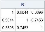
You can see that several off-diagonal elements of A were too large. The (1,2) and (2,3) elements of B are smaller than the corresponding elements of A.
Step 3: Use the positive definite matrix in your algorithm
If B is an acceptable alternative to A, you can use the B matrix instead of A. For example, if you are trying to simulate random multivariate normal data, you must use a positive definite matrix. To simulate 1,000 random trivariate observations, you can use the following function:
mean = {-2,4,0};
x = RandNormal(1000, mean, B); |
What if there are still problems?
For large matrices (say, more than 100 rows and columns), you might discover that the the numerical computation of the eigenvalues of B is subject to numerical rounding errors. In other words, if you compute the numerical eigenvalues of B, there might be some very small negative eigenvalues, such as -1E-14. If this interferes with your statistical method and SAS still complains that the matrix is not positive definite, then you can bump up the eigenvalues by adding a small multiple of the identity to B, such as B2 = ε I + B, where ε is a small positive value chosen so that all eigenvalues of B2 are positive. Of course, B2 is not a correlation matrix, since it does not have ones on the diagonal, so you need to convert it to a correlation matrix. It turns out that this combined operation is equivalent to dividing the off-diagonal elements of B by 1+ε, as follows:
/* for large matrices, might need to correct for numerical rounding errors */ epsilon = 1e-10; B2 = ProjU( B/(1+epsilon) ); /* divide off-diagonal elements by 1+epsilon */ |
How fast is Higham's algorithm?
Because each iteration of Higham's algorithm requires an eigenvector decomposition, Higham's algorithm will not be blazingly fast for huge matrices. Still, the performance is not too bad. On my desktop machine from 2010, the algorithm can project a 200 x 200 matrix in less than two seconds. You can use the TIME function to time a SAS/IML computation:
c = ranuni(j(200,200)); /* random matrix */ c = (c+c`)/2; /* symmetric matrix */ t0 = time(); /* begin timing */ R = NearestCorr(c); ElapsedTime = time()-t0; /* elapsed time, in seconds */ print ElapsedTime; |


13 Comments
Hi Rick,
This code is correct, however in practice the tolerance will allow a resulting matrix that is very close, however not quite positive semidefinite, which causes things like proc copula to reject it. I solved this problem by replacing the following line
V = choose(D>0, D, 0);
with
V = choose(D>.0001, D, .0001);
This projects the matrix inside the space of positive semidefinite matrices, instead of on the boundary, which consistently produces positive semidefinite (or most likely positive definite) output.
Thanks for this code,
Mark
You are correct. In my book Simulating Data with SAS [p. 193], I recommend leaving the projection function as it is and correcting the return matrix by using a ridging factor.
Could you explain what a ridging factor is?
A ridging factor is a multiple of the identity matrix. The magnitude of the ridging factor is the value 'epsilon' in the equation that you say does not work.
I am creating an example for an economic capital model, and am using the below code (with the above functions) to generate the matrix. Let me know if I am doing something wrong.
A = I(10); /* Allocate space for matrix */
call randgen(A,'UNIFORM'); /* Generate random numbers */
A = A + A`; /* Make matrix symmetric */
A = corr(A); /* Treat A as covariance matrix and get corr matrix */
print A;
B = NearestCorr(A); /* Find nearest pos-def corr matrix */
epsilon = 1e-10;
B2 = ProjU( B/(1+epsilon) );
print B;
For completeness, use CALL RANDSEED(1);
Your code looks fine, except that you are printing B instead of B2. B2 is symmetric, positive definite (print (eigval(B2));), and has unit diagonal.
Also, this didn't seem to work:
epsilon = 1e-10;
B2 = ProjU( B/(1+epsilon) );
Pingback: The Nearest Correlation Matrix | Nick Higham
Pingback: The arithmetic-geometric mean - The DO Loop
Hi Rick, Have you seen this recent paper by Niels Waller in TAS?
https://doi.org/10.1080/00031305.2017.1401960
He references Higham (2002) and uses a very similar algorithm to find random correlation matrices with a fixed set of eigenvalues. Thought you might like it as it has possible applications to simulating data.
Thanks for the reference. I will look at it. Regarding simulation, you can sample from a Wishart distribution that has a given spectrum is you want a statistical sample of matrices. You can also simulate random matrices that have exactly a specified set of eigenvalues.
A slight modification of the program makes it useful when you *do* require some structure in the final correlation matrix. In the example, suppose r = .99 seems too high to believe, but .35 and .80 are credible. Add these lines after Y = ProjU(X); to make these values part of Y, and eventually B:
y[3,1] = a[3,1];
y[3,2] = a[3,2];
y = sqrvech(vech(y));
The first two lines constrain values below the diagonal, and the third line makes Y symmetric. (See https://blogs.sas.com/content/iml/2012/03/21/creating-symmetric-matrices-two-useful-functions-with-strange-names.html.) Then B becomes:
1 .842 .35
.842 1 .8
.35 .8 .842
To three decimal places, r = .842 is the maximum possible correlation between the first two variables, given the other correlations. At the other extreme, changing .99 to -1 in A gives the minimum possible correlation of -.282. Ranges like this are easy to calculate when one of three correlations is missing, but much harder in larger matrices.
Thanks as always for your useful blog.
Pingback: Generate correlation matrices with specified eigenvalues - The DO Loop