In my statistical analysis of coupons article, I presented a scatter plot that includes the identity line, y=x. This post describes how to write a general program that uses the SGPLOT procedure in SAS 9.2. By a "general program," I mean that the program produces the result based on the data, not by hard-coding parameters for a specific example. I also want the program to work for a general line of the form y = a + bx.

Vertical and horizontal lines are easy to create by using the REFLINE statement in the SGPLOT procedure. Diagonal lines are a little harder. My approach is to use the VECTOR statement. See the end of this post for other ways to accomplish this task.

Editor's Note: In SAS 9.3, the SGPLOT procedure supports a LINEPARM statement. See my next article for how to add a diagonal line in SAS 9.3 or later.

The Problem and a Solution

The reason that this is not a trivial task is that the VECTOR statement will expand the plot axes if you are not careful. For example, if I plot a vector from (-600, -700) to (800, 900), the X axes will be expanded to [-600, 800] and the Y axis to [-700, 900]. A solution to this, which is due to my colleague Sanjay Matange, is to use the MIN= and MAX= options in the XAXIS and YAXIS statements to maintain the axis view ranges that are determined by the X and Y data in the scatter plot. This results in "clipping" the diagonal line so that it does not extend beyond the range of the data.

The outline of the algorithm is as follow:

1. Find the minimum and maximum values of the data that you are plotting. This is equivalent to finding the top, bottom, left, and right sides of the (eventual) scatter plot.
2. Store those values in macro variables. They will be used later by the XAXIS and YAXIS statements.
3. Store the first point of the diagonal line segment in macro variables.
4. Write the last point of the diagonal line segment to a data set. These values and the values in Step 3 will be used by the VECTOR statement.
5. Concatenate the original data with the data set in Step 4.
6. Use the SGPLOT procedure to plot the scatter plot and diagonal line, by using the data set created in Step 5.

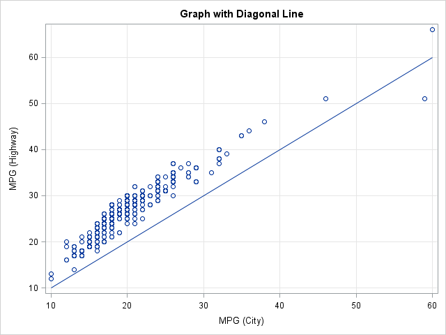
The data for this example are in the SASHELP.Cars data set. I will create a scatterplot of the MPG_CITY and MPG_HIGHWAY variables, and add the identity line. Vehicles above the line get better fuel economy on the highway than they do in the city. The final graph looks like the following:

1. Find the min and max of the data

The following SAS/IML statements read the data and compute the minimum and maximum values of the X and Y variables:

proc iml;
use sashelp.cars; /** read data **/
read all var {MPG_City} into x;
read all var {MPG_Highway} into y;
close sashelp.cars;
 
/** 1. Find min and max of data **/
xMin = min(x); xMax = max(x);
yMin = min(y); yMax = max(y);

2. Store the values in macro variables

I'm going to use these values on the XAXIS and YAXIS statements in PROC SGPLOT, so I need to get the variables out of the SAS/IML variables and into macro variables. In the SAS/IML language, you can use the SYMPUT subroutine to store a value into a macro variable. (When putting a numeric value into a macro variable, I use the CHAR or PUTN functions to convert the value to a character string.) The following statements store the values into macro variables of the same name:

/** 2. Store as macro variables **/
call symput("xMin", char(xMin));
call symput("xMax", char(xMax));
call symput("yMin", char(yMin));
call symput("yMax", char(yMax));

3. Store the first point in macro variables

/** Linear helper function **/
start L(x);
   a = 0; /** intercept **/
   b = 1; /** slope **/
   return(a + b#x);
finish;
 
/** 3. Store the origin in macro variables **/
call symput("x0", char(xMin));
call symput("y0", char(L(xMin)));

4. Write the last point to a data set

Because of the syntax of the VECTOR statement, you need to write the final point of the line segment to a SAS data set. This data set will be concatenated with the original data in the next step of the algorithm. The following statements create the EndLine data set, which consists of two variables (LX and LY) and a single observation:

/** 4. Write vars LX and LY to data set **/
Lx = xMax; Ly = L(xMax); 
create EndLine var {Lx Ly};
   append;
close EndLine;

5. Concatenate the data sets

The original data are in SASHELP.cars. I want to add two new variables, XF and YF, which contain the endpoint of the diagonal line segment. The following data step adds the variables:

data cars;
   set sashelp.cars EndLine;
run;

Notice that the CARS data set has a block structure. The first 428 observations are a copy of the SASHELP.Cars data, except that there are two new variables, LX and LY, which have missing values. The final observation (#429) has missing values for all of the variables in the SASHELP.Cars data set, but has nonmissing values for the LX and LY variables.

6. Create the plot

The following statements use the SGPLOT procedure to create a scatter plot. A diagonal line is overlaid by using the VECTOR statement.

proc sgplot data=cars noautolegend;
   title "Graph with Diagonal Line";
   scatter x=MPG_City y=MPG_Highway;
   vector x=Lx y=Ly / xorigin=&x0 yorigin=&y0 noarrowheads;
   xaxis grid min=&xMin max=&xMax;
   yaxis grid min=&yMin max=&yMax;
run;

Other Ways to Overlay Diagonal Lines

If you use the Graph Template Language (GTL), you can use the LINEPARM statement to overlay a line with a specified slope. This is probably an easier technique if you are comfortable with the GTL.

In the SGPLOT procedure, you could also use the SERIES statement, rather than the VECTOR statement. Use the SERIES statement when you want to overlay a curve that is not a straight line.

In SAS 9.3, the SGPLOT procedure will support a LINEPARM statement. In addition, SAS 9.3 supports an annotation facility, as described in Dan Heath's SAS Global Forum 2011 paper.

If you want to learn more about the many graphs that you can create by using the SGPLOT procedure, I recommend the SGPLOT Gallery. I also recommend looking at a copy of Sanjay and Dan's forthcoming book, Statistical Graphics Procedures by Example, which will be published in Fall 2011.