Readers' comments indicate that my previous blog article about computing the area under an ROC curve was helpful. Great! There is another common application of numerical integration: finding the area under a density estimation curve.

This article provides an overview of density estimation and computes an empirical cumulative density function. Future articles will describe parametric and nonparametric density estimation.

The Importance of Density Estimation and Integration

Density estimation is the process of using observed data to construct an estimate to the probability density function of a random variable (Silverman, 1992, p. 1). Statisticians know that the area under a probability density function gives information about the probability that an event occurs. The simplest density estimate is a histogram, but you can also estimate the density by fitting parametric curves (for example, a normal curve) or nonparametric curves (for example, a kernel density estimate curve) to the observed data.

For example, if you sample the cholesterol of N women, you can use that information to estimate the probability that the cholesterol of a random woman in the population is less than 200 mg/dL (desirable), or greater than 240 mg/dL (high), or between any two specified values.

To be concrete, consider the cholesterol of 2,873 women in the Framingham Heart Study as recorded in the SAS data set SASHELP.Heart, which is distributed with SAS/GRAPH software in SAS 9.2. You can use the UNIVARIATE procedure to construct a histogram and various parametric and nonparametric density estimates of the cholesterol variable. The following statements use the VSCALE= option to set the vertical scale of the histogram to the density scale:

data FHeart;
set sashelp.heart; where sex="Female";
run;
 
ods graphics on;
proc univariate data=FHeart;
   var cholesterol;
   histogram / vscale=proportion
             normal kernel(C=SJPI);
run;

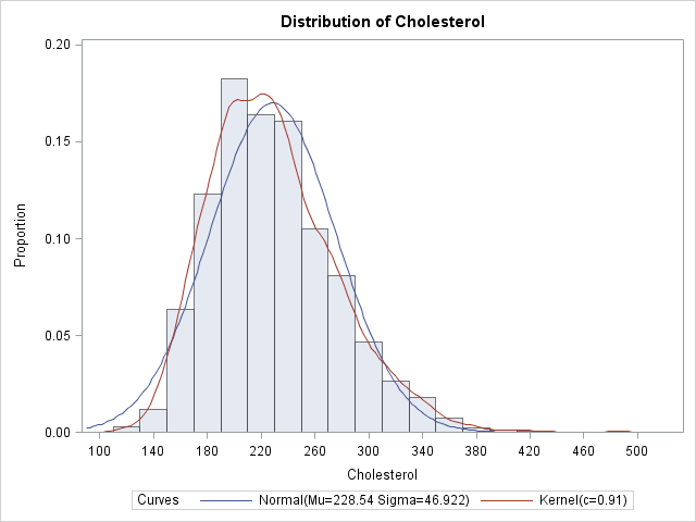
The histogram is a density estimate, as are the normal and kernel density curves. Each can be used to estimate the probability that the cholesterol of a random woman in the population is within a certain range of values.

Empirical Estimates from the Data

You can sum the areas of the first k histogram bars in order to estimate the probability that a random woman has cholesterol less than the right endpoint of the kth bar. For example, an estimate of the probability that a random woman has cholesterol less than 190 mg/dL (the right endpoint of the fourth bar) is about 20.2. However, it is often more convenient to use the data directly to estimate the proportion of the population that satisfies certain conditions. As I've written before, it is easy to use the SAS/IML language to find data that satisfy some criterion. For example, the following statements read in the cholesterol data into a SAS/IML vector, x, and compute the proportions of the data that are less than 200 mg/dL and greater than 240 mg/dL:

proc iml;
use FHeart;
read all var {cholesterol} into x;
close FHeart;
 
/** x contains missing values **/
x = x[loc(x^=.)]; /** remove missing **/
 
N = nrow(x);
lt200 = sum(x<200) / N;
ge240 = sum(x>=240)/ N;
print N lt200 ge240;

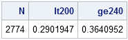
In the data, 29% of the women have cholesterol less than 200 and 36% of the women have cholesterol greater than or equal to 240 mg/dL. If you believe that the women in the study are representative of women in the general population, you can use these values to estimate the corresponding proportions in the population.

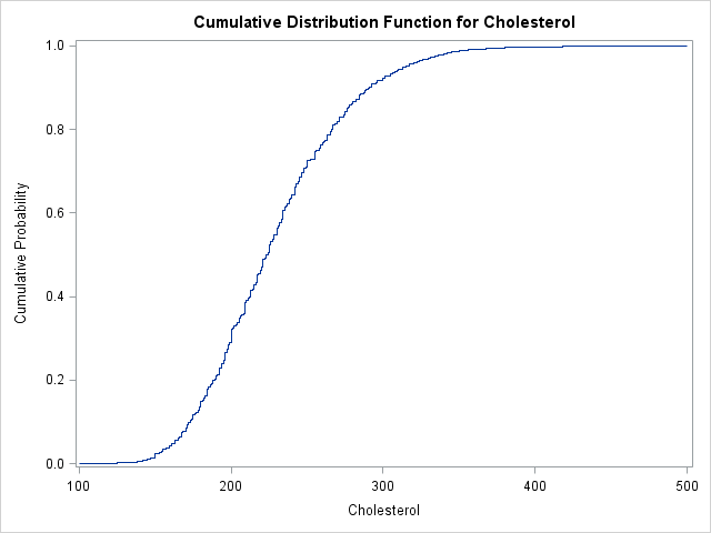
The Empirical Cumulative Distribution Function

The value 200, although "special" for medical reasons, is not special in a mathematical sense. You can compute the proportion of observations in the data that are less than 180, 221, or any other value. If you compute the proportion of observations in the data that are less than or equal to c for all possible values of c, then you have computed the points on the empirical cumulative distribution function (ECDF). The ECDF is a step function increases by 1/N at each observed data value.

It is easy to use the SAS/IML language to compute the points on the ECDF. One approach is to use the UNIQUE function to find a sorted list of the unique values of x, and then loop over those unique values to compute the proportion of observations that are less than each value:

u = unique(x);
ecdf = j(1, ncol(u));
do i = 1 to ncol(u);
   ecdf[i] = sum(x<=u[i]); /** counts **/
end;
ecdf = ecdf / N; /** normalize **/

You can write the U and ECDF vectors to a SAS data set and plot the ECDF with the SGPLOT procedure. Alternately, you can use the CDFPLOT statement of the UNIVARIATE procedure to compute and plot the ECDF directly from the data:

proc univariate data=FHeart;
   var cholesterol;
   cdfplot / vscale=proportion
run;