The area under a density estimate curve gives information about the probability that an event occurs. The simplest density estimate is a histogram, and last week I described a few ways to compute empirical estimates of probabilities from histograms and from the data themselves, including how to construct the empirical cumulative density function (ECDF).

This article describes how to estimate the density by fitting a parametric curve (for example, a normal curve) to the observed data.

Fitting a Parametric Density Estimate to Data

You can use the UNIVARIATE procedure to fit the parameters in a model to data. The UNIVARIATE procedure supports a large number of well-known distributions, and not only fits the model for you (using, typically, a maximum likelihood optimization), but can also graph the results by using ODS statistical graphics.

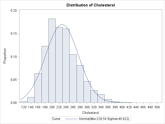
I will use the same example that I used in my previous article: the cholesterol of 2,873 women in the Framingham Heart Study as recorded in the SAS data set SASHELP.Heart, which is distributed with SAS/GRAPH software in SAS 9.2. The cholesterol data are approximately normal, so I will fit a normal curve to the data to illustrate the technique. You can use the UNIVARIATE procedure to create three relevant items:

• a histogram and a normal density estimate to the data
• a graph of the parametric and empirical CDF (not shown)
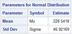
• a table of parameter estimates

The parameter estimates are necessary in order to compute the area under the parametric PDF, so the following statements use the ODS OUTPUT statement to write the ParameterEstimates table to a SAS data set named PE:

data FHeart;
set sashelp.heart; where sex="Female";
run;
 
ods graphics on;
proc univariate data=FHeart;
   ods output ParameterEstimates=PE;
   var cholesterol;
   histogram / vscale=proportion normal;
   cdfplot / normal;
run;

The UNIVARIATE procedure creates the parameter estimates table, as follows:

The Area under a Parametric Density Estimate Curve

You can use the parameter estimates to estimate the probability that a random woman has cholesterol less than 200 mg/dL (desirable) and greater than 240 mg/dL (high). Simply read in the parameter estimates into the SAS DATA step or the SAS/IML language, and use the CDF function in Base SAS to integrate the fitted curve. The following SAS/IML statements read the parameter estimates and compute two areas: the area under the fitted curve that is less than 200, and the area that is greater than 240:

proc iml;
use PE;
read all var {Estimate};
close PE;
 
mu = Estimate[1];
sigma = Estimate[2];
lt200 = cdf("Normal", 200, mu, sigma);
ge240 = 1 - cdf("Normal", 240, mu, sigma);
print lt200 ge240;

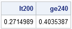
The value of LT200 represents an estimate of the probability that a random woman in the population has cholesterol less than 200. The value of GE240 is an estimate of the probability that a random woman has cholesterol greater than 240. These estimates assume that the distribution of cholesterol in women in the population is normally distributed, which is probably not the best model, based on the skewness of the histogram and the goodness-of-fit test that PROC UNIVARIATE displays (not shown here).

Notice that to compute GE240, you use the CDF function to compute the area less than 240 and then subtract that value from the total area under the curve, which is 1.

This parametric method estimates that 27% of women have cholesterol less than 200, and 40% have cholesterol greater than 240. Although the normal model might not be suitable for these data, these parametric estimates are not too different from the empirical estimates that were computed in the previous article.