Statistical programmers often need to evaluate complicated expressions that contain square roots, logarithms, and other functions whose domain is restricted. Similarly, you might need to evaluate a rational expression in which the denominator of the expression can be zero. In these cases, it is important to avoid evaluating a function at any point that is outside the function's domain.

This article shows a technique that I call "trap and cap." The "trap" part of the technique requires using logical conditions to prevent your software from evaluating an expression that is outside the domain of the function. The "cap" part is useful for visualizing functions that have singularities or whose range spans many orders of magnitude.

This technique is applicable to any computer programming language, and it goes by many names. It is one tool in the larger toolbox of defensive programming techniques.

This article uses a SAS/IML function to illustrate the technique, but the same principles apply to the SAS DATA step and PROC FCMP. For an example that uses FCMP, see my article about defining a log transformation in PROC FCMP.

ERROR: Invalid argument to function

The following SAS/IML function involves a logarithm and a rational expression. If you naively try to evaluate the function on the interval [-2, 3], an error occurs:

proc iml;
/* Original function module: No checks on domain of function */
start Func(x);
   numer = exp(-2*x) # (4*x-3)##3 # log(3*x);       /* not defined for x <= 0 */
   denom = x-1;                                     /* zero when x=1 */
   return( numer / denom );
finish;
 
x = do(-2, 3, 0.01);
f = Func(x);

ERROR: (execution) Invalid argument to function.

 count     : number of occurrences is 200
 operation : LOG at line 881 column 40

The error says that there were 200 invalid arguments to the LOG function. The program stops running when it encounters the error, so it doesn't encounter the second problem, which is that the expression numer / denom is undefined when denom is zero.

Experienced SAS programmers might know that the DATA step automatically plugs in missing values and issue warnings for the LOG function. However, I don't like warnings any more than I like errors: I want my program to run cleanly!

Trap bad input values

Because the function contains a logarithm, the function is undefined for x ≤ 0. Because the function is a rational expression and the denominator is zero when x = 1, the function is also undefined at that value.

The goal of the "trap" technique is to prevent an expression from being evaluated at points where it is undefined. Accordingly, the best approach is to compute the arguments of any function that has a restricted domain (log, sqrt, arc-trigonometric functions,...) and then use the LOC function to determine the input values that are within the domain of all the relevant functions. The function is only evaluated at input values that pass all domain tests, as shown in the following example:

proc iml;
/* Trap bad domain values; return missing values when x outside domain */
start Func(x);
   f = j(nrow(x), ncol(x), .);    /* initialize return values to missing */
   /* trap bad domain values */
   d1 = 3*x;                      /* argument to LOG */
   d2 = x-1;                      /* denominator */
   domainIdx = loc( d1>0 & d2^=0 );     /* find values inside domain */
   if ncol(domainIdx)=0 then return(f); /* all inputs invalid; return missing */
 
   t = x[domainIdx];              /* elements of t are valid */
   numer = exp(-2*t) # (4*t-3)##3 # log(3*t);
   denom = t-1;
   f[domainIdx] = numer / denom;  /* evaluate f(t) */
   return( f );
finish;
 
x = do(-2, 3, 0.01);
f = Func(x);

This call does not encounter any errors. The function returns missing values for input values that are outside its domain.

In practice, I advise that you avoid testing floating-point numbers for equality with zero. You can use the ABS function to check that quantities are not close to zero. Consequently, a preferable trapping condition follows:

   domainIdx = loc( d1>0 & abs(d2)>1e-14 );  /* find values inside domain */

I also recommend that you use the CONSTANT function to check for domain values that would result in numerical underflows or overflows, which is especially useful if your expression contains an exponential term.

Cap it! Graphing functions with singularities

You have successfully evaluated the function even though it has two singularities. Let's see what happens if you naively graph the function. The function has a horizontal asymptote at y=0 and vertical asymptotes at x=0 and x=1, so you can use the REFLINE statement in PROC SGPLOT to draw reference lines that aid the visualization. In SAS/IML, you can use the SCATTER subroutine to create a scatter plot, and pass the REFLINE statements by using the OTHER= option, as follows:

refStmt = "refline 0/axis=y; refline 0 1/axis=x;"; /* add asymptotes and axes */
call scatter(x, f) other=refStmt;

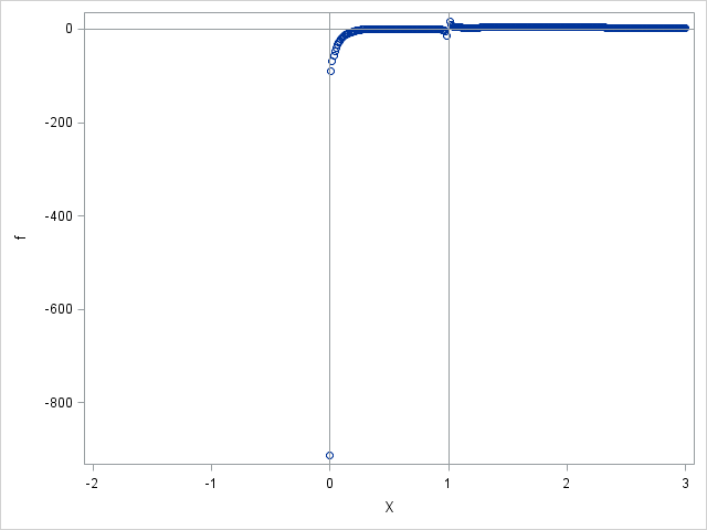
The graph is not very useful (look at the vertical scale!) because the magnitude of the function at one point dwarfs the function values at other points. Consequently, you don't obtain a good visualization of the function's shape. This is often the case when visualizing a function that has singularities.

/* cap the view at +/-5 */
title "Sketch of Function";
title2 "-5 < y < 5";
capStmt = "yaxis min=-5 max=5;";
call scatter(x,f) other=capStmt + refStmt;

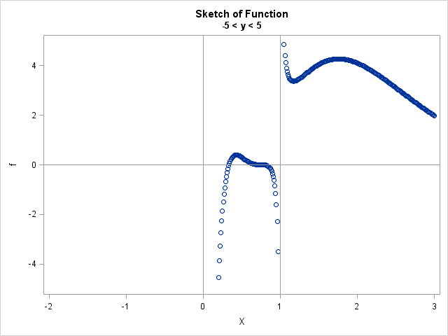
This latest graph provides a good overview of the function's shape and behavior. For intervals on which the function is continuous, you can get a nicer graph if you use the SERIES subroutine to connect the points and hide the markers. The following statements re-evaluate the function on the interval (0, 1) and caps the vertical scale by using -1 < y < 1:

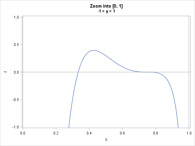
title "Zoom into [0, 1]";
title2 "-1 < y < 1";
x = do(0, 1, 0.01);
f = Func(x);
capStmt = "yaxis min=-1 max=1;";
call series(x,f) other=capStmt + refStmt;

The resulting graph shows that the function has two roots in the interval (0, 1) and a local maximum near x=0.43. A visualization like this is often an important step in finding the roots or local extrema of a function.

In summary, the trap-and-cap technique enables you evaluate functions that have singularities or that have a restricted domain. For SAS/IML functions, you can use the LOC function to keep only the input values that are in the domain of the function. (In a scalar language, such as the SAS DATA step, you can use IF-THEN/ELSE statements instead.) For functions with singularities, you can use the YAXIS statement in PROC SGPLOT to ensure that a graph of the function reveals interesting features and not just extreme values.