Nonlinear optimization routines enable you to find the values of variables that optimize an objective function of those variables. When you use a numerical optimization routine, you need to provide an initial guess, often called a "starting point" for the algorithm. Optimization routines iteratively improve the initial guess in an attempt to converge to an optimal solution. Consequently, the choice of a starting point determines how quickly the algorithm converges to a solution and—for functions with multiple local extrema—to which optimum the algorithm converges.
But how can you produce a "good" starting point for multivariate functions? Some analysts use a constant vector, such as a vector of all 0s or a vector of all 1s. Although this practice is widespread, this default initial guess might not converge to a global extremum. You can usually do better by choosing a starting point that is based on a few easy evaluations of the objective function.
I recently described how to use the EXPANDGRID function in SAS/IML software to construct a set of ordered k-tuples that are arranged on a uniformly spaced grid. By evaluating a function on a grid, you can visualize the function and determine a starting point for an optimization algorithm. This "evaluate on a grid" technique is sometimes called a "pre-search" technique. This article shows how to choose an initial guess when there are no constraints on the parameters of the objective function ("unconstrained optimization").
Defining objective functions in SAS/IML
To use the pre-search technique, you should write your objective function so that you can pass in a matrix. The columns of the matrix are the variables in the equation for the objective function. Each row of the matrix is a point at which to evaluate the function.
The NLP routines in SAS/IML will work even if your objective function evaluates only scalar values, but the pre-search technique is much more efficient if you write a vectorized function. To vectorize a function, use the elementwise multiplication operator (#) in your formulas. For example, if your objective function is g(x,y) = x2 + x*y + y2, define the following SAS/IML function:
proc iml;
start g(m);
   x = m[,1]; y = m[,2];        /* variables are columns of m */
   return( x##2 + x#y + y##2 ); /* use elementwise multiplication */
finish;

m = {0 0,     /* test it: define three points in the domain of g */
     0 1,
     1 2};
z = g(m); /* one call evaluates g(x,y) at three points! */ |
By writing the function in a vectorized fashion, you can evaluate arbitrarily many points (rows of a matrix) with a single call.
Visualizing a function of two variables
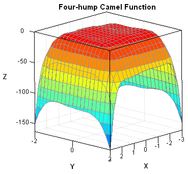
There are several "test suites" of functions that are used to test optimization algorithms. One test function is called the "four-hump camel function" because it has four local maxima (from Dixon and Szego (1978), "The global optimization problem: an introduction"). Some people call it the "six-hump camel function" because it also has two local minima, but that's a misnomer. The camel function is a polynomial equation in two variables:
f(x,y) = (4 - 2.1 x2 + x4 /3) x2 + xy +
(-4 + 4 y2) y2
The following SAS/IML function defines the four-hump camel function, generates a uniform grid of points on the rectangle [–3, 3] x [–2, 2], and creates a rotating surface plot by using the RotatingPlot graph in the SAS/IML Studio application:
proc iml;
/* four-hump camel has two global maxima:
   p1 = {-0.08984201  0.71265640 };
   p2 = { 0.08984201 -0.71265640 };   */
start Camel(m);
   x = m[,1];  y = m[,2];
   f = ( 4 - 2.1*x##2 + x##4 /3) # x##2 + x#y +
       (-4 + 4  *y##2) # y##2;
   return( -f );   /* return -f so that extrema are maxima */
finish;

m = ExpandGrid( do(-3, 3, 0.1), do(-2, 2, 0.1) );   /* SAS/IML 12.3 */
z = Camel(m);

/* In SAS/IML Studio, visualize surface with 3D rotating plot */
RotatingPlot.Create("Camel", m[,1], m[,2], z); |
The surface plot is shown at the top of this article. It indicates that the function is fairly flat on top, but has small bumps that contain local maxima. By using the interactive graphics in SAS/IML Studio, it is easy to find the absolute maxima (there are two), or you can find the maxima programmatically by using the following statements:
optIndex = loc(z=max(z)); /* find maximum values of z */ optX = m[optIndex,]; /* corresponding (x,y) values */ print optX; |

Prior to these computations, I had never seen the "camel function" before. I did not know where the maxima might be. However, by evaluating the function on a coarse grid of 2,500 points, I now know that if I want to find global maxima, I should look in a neighborhood of (–0.1, 0.7) and (0.1, –0.7). These would be good choices to use as starting points for an optimization algorithm.
Visualizing a function of three variables
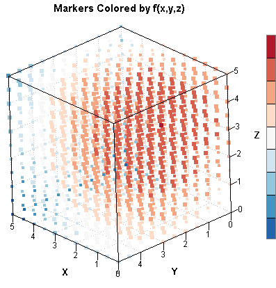
Although it is harder to visualize a function of three variables (the graph is in four-dimensional space!), you can still get a feel for high and low values of a function. You can evaluate a function of three variables on a uniform grid and then color each point in the grid according to the functional value at that point. This generalizes the two-dimensional example that I wrote about in the article "Color scatter plot markers by values of a continuous variable." As an example, define the following quadratic function:
Q(x,y,z) = –(x - 1.1)2 – (y - 2.2)2 – (z - 3.3)2
By inspection, the function Q(x,y,z) has a single global maximum at the point (1.1, 2.2, 3.3). The following statements evaluate the function on a 3-D grid of half integers:
start Q(x); return( -(x[,1] - 1.1)##2 - (x[,2] - 2.2)##2 - (x[,3] - 3.3)##2 ); finish; m = ExpandGrid( do(0,5,0.5), do(0,5,0.5), do(0,5,0.5) ); f = Q(m); optIndex = f[<:>]; /* find maximum values of Q */ optX = m[optIndex,]; /* corresponding (x,y,z) values */ print optX; |

The result shows that (1, 2, 3.5) is the point on the grid for which the function is the largest. If you start a numerical optimization from that point, you will converge very quickly to the optimal solution. The 3-D scatter plot at the beginning of this section is a scatter plot of the grid, where each point has been colored according to the value of Q. The big blob of red indicates where the function is the largest. This graph crudely visualizes the function by showing where it is large and where it is small.
Finding an initial guess for an extremum
In theory, the pre-search technique works for any multivariate function. However, the size of the grid grows geometrically as the number of variables increases, so you will need to reduce the coarseness of the grid for functions of many variables. For example, if you use k grid points for each variable of a 10-dimensional function, then the grid will contain k10 points! Clearly, you should choose k to be small. If k = 5, then the grid contains 510 = 9.7 million points, which is large, but still computationally manageable. For functions with more than 15 variables, the pre-search technique on a "full factorial" grid becomes impractical.
Nevertheless, a coarse grid gives you more information than no grid at all, and a starting point based on the pre-search technique is usually superior to an arbitrary starting point. It is easy to implement the pre-search technique in the SAS/IML language, and you can often use it to provide a good initial guess to a nonlinear optimization routine.

8 Comments
is this possible for constrained optimization?
An excellent question! Yes, you can form a uniform grid of points and then evaluate each point to see whether it is feasible (=satisfies constraint). Throw out the infeasible points, and evaluate the function only on the feasible points.
Hi Rick,
I am working on an optimization problem including 9 parameters for the objective function. The problem is also constraints. I am wondering how I can find domains for each variable in "ExpandGrid" statement?
I have no idea how the grid spaces and borders should be determined.
I appreciate any help,
Azam
This can be a tricky problem. For linear constraints and boundaries, you can use the NLPFEA subroutine.
Pingback: Ten tips before you run an optimization - The DO Loop
Pingback: Grids and linear subspaces - The DO Loop
Pingback: How to find a feasible point for a constrained optimization in SAS - The DO Loop
Pingback: How to find a feasible point for a constrained optimization in SAS - The DO Loop