Last week I wrote about using acceptance-rejection algorithms in vector languages to simulate data. The main point I made is that in a vector language it is efficient to generate many more variates than are needed, with the knowledge that a certain proportion will be rejected.
In last week's article, I used a zero-truncated Poisson distribution as an example of a random variable that can be generated by using an acceptance-rejection algorithm. If you generate a random variate from a Poisson(λ=0.5) distribution, the probability that the generated value is nonzero is 0.3935. The Poisson(0.5) distribution is sometimes called the instrumental distribution. It is the distribution from which you unconditionally generate data.
You might attempt to generate 1000 / 0.3935 = 2,542 Poisson(0.5) variates, in hopes of obtaining 1,000 that are positive. The problem with this idea is that an expected value is not a guaranteed value! In last week's article I ran a single simulation in which I asked for 2,542 Poisson variates, and 1,009 of those turned out to be positive. However, basically I got lucky. The following graph shows the result of repeating that simulation many times. The histogram shows the number of positive values that are generated each time that I generate 2,542 variates from the instrumental distribution. You can see that although the expected number of positive variates is 1,000 (as shown by the mean of the histogram), you might get unlucky and obtain as few as 920 positive values.
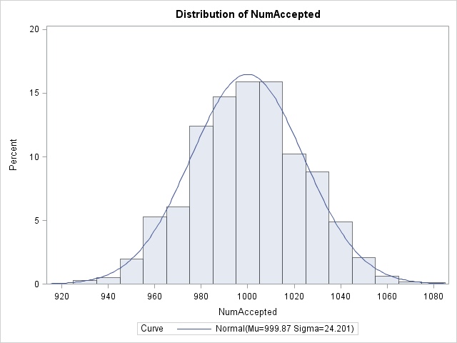
The graph shows the sampling distribution of the number of positive variates that you obtain when you generate 2,542 Poisson(0.5) variates. The graph suggests an easy modification: shift the graph to the right by asking for EVEN MORE variates from the instrumental distribution! In particular, ask for enough to be 99.9% certain that you will obtain at least 1,000 positive variates.
There are a couple of ways to implement this approach. The most straightforward is to recognize that the histogram is an approximation of the binomial distribution, Binom(p, M), where p=0.3935 is the probability of "success" (acceptance) and M is the number of instrumental variates that you generate. Therefore, you can define a vector of values of M, and find a value of M such that there is less than a 0.1% chance of obtaining fewer than 1,000 positive values:
proc iml;
p = 0.3935;
MM = 2700:2800;        /* range of values for M */
q = quantile("Binomial", 0.001, p, MM);
idx = loc(q>=1000);    /* find all M for which P(X<1000) is tiny */
if ncol(idx) > 0 then do;
   M = v[idx][1];      /* extract first (smallest) values */
   print M;
end; |
The computation says that if you ask for M = 2,741 Poisson(0.5) variates, that there is a 99.9% chance that at least 1,000 of them will be positive. (For this example, you could also use the normal approximation to the binomial distribution.)
An even more efficient solution is to use the negative binomial distribution. The event "accept or reject a Poisson(0.5) variable" is a Bernoulli random variable with the probability of "success" equal to p=0.3935. The negative binomial is the distribution of the number of failures before k successes in a sequence of independent Bernoulli trials. You can compute F, the 99.9th percentile of the number of failures that you encounter before you obtain 1,000 successes. The total number of trials that you need is therefore F + 1000:
F = quantile("NegBinomial", 0.999, p, 1000);
M = F + 1000;
print F M; |

Same answer. Same interpretation.
Although I have discussed these issues for the particular example of simulating N observations from a zero-truncated Poisson distribution, the same approach is generally applicable. In many acceptance-rejection algorithms you can compute the probability of the "acceptance" event. "Acceptance" is therefore a Bernoulli random variable with probability p, so you can use the quantiles of the negative binomial distribution to compute how many variates you will need to generate from the instrumental distribution before N values are accepted.

1 Comment
Pingback: Efficient acceptance-rejection simulation - The DO Loop