Polynomials are used often in data analysis. Low-order polynomials are used in regression to model the relationship between variables. Polynomials are used in numerical analysis for numerical integration and Taylor series approximations. It is therefore important to be able to evaluate polynomials in an efficient manner.
My favorite evaluation technique is known as Horner's scheme. This algorithm is amazingly simple to describe and to implement. It has the advantage that a polynomial of degree d is evaluated with d additions and d multiplications. With this scheme, you never have to explicitly raise the variable, x, to a power.
To explain Horner's scheme, I will use the polynomial
p(x) = 1x3 - 2x2 - 4x + 3.
Horner's scheme rewrites the polynomial as a set of nested linear terms:
p(x) = ((1x - 2)x - 4)x + 3.
To evaluate the polynomial, simply evaluate each linear term. The partial answer at each step of the iteration is used as the "coefficient" for the next linear evaluation.
In SAS/IML software, it is customary to store polynomial coefficients in a vector in order of descending powers of the polynomial. For example, the coefficients of the example polynomial are stored in the vector {1, -2, -4, 3}. The following SAS/IML module implements Horner's scheme for evaluating a polynomial at a set of points:
proc iml;
start Polyval(coef, v);
/*  Polyval(c,x) uses Horner's scheme to return the value of a polynomial of
degree n evaluated at x. The input argument c is a column
vector of length n+1 whose elements are the coefficients
in descending powers of the polynomial to be evaluated.
The input argument x can be a vector of values. */
   c = colvec(coef); x = colvec(v); /* make column vectors */
   y = j(nrow(x), 1, c[1]); /* initialize to c[1] */
   do j = 2 to nrow(c);
      y = y # x + c[j];
   end;
   return(y);
finish;

/* 1*x##3 - 2*x##2 -4*x + 3 */
c = {1, -2, -4, 3};
x = do(-2, 3.5, 0.5); /* evaluate at these points */
y = Polyval(c, x);
print (x`)[label="x"] y; |
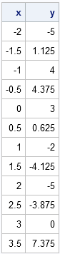
The polynomial is evaluated at a set of points in the interval [-2, 3.5]. The function values show three sign changes, indicating that the polynomial has roots (zeros) in the intervals [-2, -1.5] and [0.5, 1], and at the point x=3. As shown in my post on finding the roots of univariate functions, you can use the POLYROOT function in SAS/IML to locate the roots.
The Polyval module is efficient not only because it uses Horner's scheme to evaluate the polynomial, but also because it is vectorized: it can evaluate the polynomial at a set of points with a single call. A few comments on the implementation:
- The COLVEC module, which is part of the IMLMLIB library, converts the arguments to column vectors. That way, you can pass in row vectors, column vectors, or even matrices, and the module works correctly. Alternatively, you can have the module always output a matrix that is the same dimensions as x.
- The output vector, y, is initialized to contain c[1], the leading coefficient of the polynomial. The y vector contains the same number of elements as the x vector.
- The fact that the module accepts a vector of x values is almost hidden. The only hints are that y is allocated to be a vector and the elementwise multiplication operator (#) is used within the DO loop.

3 Comments
Pingback: Approximate functions by using Taylor series and rational polynomials - The DO Loop
Pingback: On the evaluation of the function exp(x) - 1 - The DO Loop
Pingback: Create an interpolating polynomial in SAS - The DO Loop