One of the joys of statistics is that you can often use different methods to estimate the same quantity. Last week I described how to compute a parametric density estimate for univariate data, and use the parameters estimates to compute the area under the probability density function (PDF). This article describes how to compute a kernel density estimate (KDE) and to integrate that curve numerically.
Some practicing statisticians (especially those over a certain age!) learned parametric modeling techniques in school, but later incorporated nonparametric techniques into their arsenal of statistical tools. A very common nonparametric technique is kernel density estimation, in which the PDF at a point, x is estimate by a weighted average of the sample data in a neighborhood of x. Kernel density estimates are widely used, especially when the data appear to be multi-modal.
Kernel Density Estimation in SAS
As before, consider the cholesterol of 2,873 women in the Framingham Heart Study as recorded in the SAS data set SASHELP.Heart, which is distributed with SAS/GRAPH software in SAS 9.2. You can use the UNIVARIATE procedure to construct a kernel density estimate for the cholesterol variable.
The kernel density estimator has a parameter (called the bandwidth) that determines the size of the neighborhood used in the computation to compute the estimate. Small values of the bandwidth result in wavy, wiggly, KDEs, whereas large values result in smooth KDEs. The UNIVARIATE procedure has various methods to select the bandwidth automatically. For this example, I use the Sheather-Jones plug-in (SJPI) bandwidth.
The following statements use the OUTKERNEL= option to output the kernel density estimate at a sequence of regularly space values, and the VSCALE= option to set the vertical scale of the histogram to the density scale:
data heart; set sashelp.heart; where sex="Female"; run; ods graphics on; proc univariate data=heart; var cholesterol; histogram / vscale=proportion kernel(C=SJPI) outkernel=density; run; |
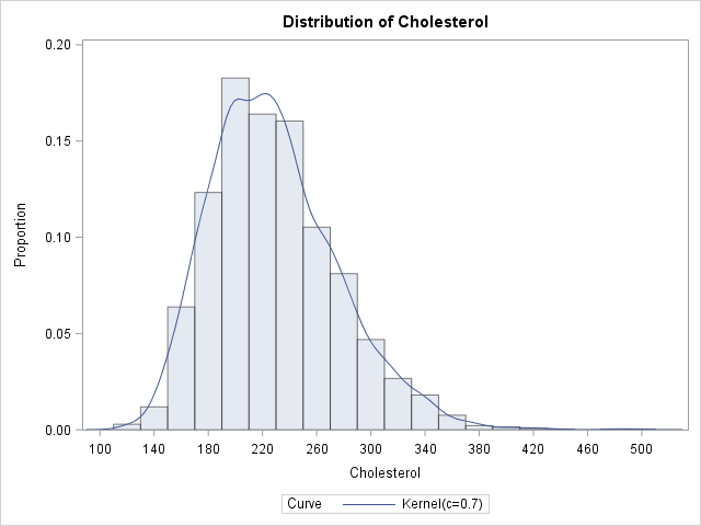
The nonparametric kernel density estimate exhibits features that are not captured by parametric models. For example, the KDE for these data show several bumps and asymmetries that are not captured by the assumption that the data are normally distributed.
The DENSITY data set contains six variables. The _VALUE_ variable represents the X locations for the density curve and the _DENSITY_ variable represents the Y locations. Therefore the area under the density estimate curve can be computed by numerically integrating those two variables.
Overcoming a Bug in the OUTKERNEL= Option in SAS 9.2
If you are using SAS 9.2, read this section. There is a bug in the OUTKERNEL= option in SAS 9.2 which results in the DENSITY data set containing two (identical) copies of the KDE curve! (The bug is fixed in SAS 9.3 and beyond.) Here's how to remove the second copy: find the maximum value of the X variable and delete all observations that come after it. The maximum value of X ought to be the last observation in the DENSITY data. The following statements read the density curve into the SAS/IML language and eliminate the second copy of the curve:
proc iml;
/** read in kernel density estimate **/
use density;
read all var {_value_} into x;
read all var {_density_} into y;
close density;

/** work around bug in OUTKERNEL data set in SAS 9.2 **/
/** remove second copy of data **/
max = max(x);
idx = loc(x=max);
if ncol(idx) > 1 then do;
  x = x[1:idx[1]];  y = y[1:idx[1]];
end; |
The previous statements remove the second copy of the data if it exists, but do nothing if the second copy does not exist. Therefore it is safe to run the statements in all versions of SAS.
The Area under a Kernel Density Estimate Curve
The kernel density estimate is not a simple function. The points on the curve are available only as a sequence of (X, Y) pairs in the DENSITY data set. Consequently, to integrate the KDE you need to use a numerical integration technique. For this example, you can use the TrapIntegral module from my blog post on the trapezoidal rule of integration.
The following statements define the TrapIntegral module and verify that the KDE curve is correctly defined by integrating the curve over the entire range of X values. The area under a density estimate should be 1. If the area is not close to 1, then something is wrong:
start TrapIntegral(x,y); N = nrow(x); dx = x[2:N] - x[1:N-1]; meanY = ( y[2:N] + y[1:N-1] )/2; return( dx` * meanY ); finish; /** compute the integral over all x **/ Area = TrapIntegral(x,y); print Area; |

Ahh! Success! The area under the KDE is 1 to within an acceptable tolerance. Now to the real task: compute the area under the KDE curve for certain medically interesting values of cholesterol. In particular, the following statements estimate the probability that the cholesterol of a random woman in the population is less than 200 mg/dL (desirable), or greater than 240 mg/dL (high):
/** compute the integral for x < 200 **/ idx = loc(x < 200); lt200 = TrapIntegral(x[idx],y[idx]); /** compute the integral for x >= 240 **/ idx = loc(x >= 240); ge240 = TrapIntegral(x[idx],y[idx]); print lt200 ge240; |
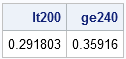
If you believe that the KDE for these data is a good estimate of the distribution of cholesterol in women in the general population, the computations show that about 29% of women have healthy cholesterol levels, whereas 36% have high levels of cholesterol. These are approximately the same values that were computed by using empirical probability estimates, as shown in my original post on this topic. They differ by about 2% from the parametric model, which assumes normally distributed data.
In practice, it is usually better to use the empirical estimates, rather than the technique used in this article, because the empirical estimates are unbiased. The KDE requires the selection of a bandwidth, and techniques such as the Sheather-Jones plug-in (SJPI) method choose the bandwidth to optimize some density-fitting criterion, not the probability estimates. If you choose a different criterion, you will get a different bandwidth, which can lead to a different probability estimate.

10 Comments
I just googled the "density estimation SAS" and this post came out the second! Very cool:) I do not know if you can do that, but IMHO the links to the social networking and bookmariking websites will serve better if they are on the top of the page as well as on the bottom.
Thanks, Peter. The SAS blogs are moving to a new Blogging Platform in a few weeks. I'm told that the social media links at the new site will be easier to access.
Dear Mr Wicklin, thanks a lot for all your interesting and extremely useful post!
Have you ever considered writing one about how to plot the difference between two kernel densities? :)
I haven't. The difference between two densities can be negative, so in particular it is not itself a density. Do you have an application in mind or a reference to a book or paper on the topic?
We are comparing the income kernel densities of non-migrants and migrants (prior to migration) and we would like to plot the difference between densities to better show the positive selection (as Jesus Moraga did in: New evidence on emigrant selection, Review of Economics and Statistics, 2011).
In R, for instance, this would be done by computing the arithmetic difference between the linear interpolation of the two kernel density functions. I am still looking for a book/paper that would provide some sort of theoretical background.
Yes, you can do that in SAS by using PROC KDE. See the example in the following article: "The Difference of Density Estimates"
The area under the density curve should be 0. Is this true for the boundary-corrected Kernel density estimation?
The area under the density curve should be 1, not 0. This should be true for all density estimates that you integrate on (-infinity, infinity).
Dear Rick,
thank you for this post.
I am conducting simulations to compare methods for cutoff estimation. One is kernel density estimation where I use the intersection of 2 pdfs as a cutoff. For these I want to estimate sensitivity and specificity or area under the curve =cutoff.
Your code works very well when I use a single sample, but I am unable to make it run over e.g. a 1000 simulations. Thus, I need to construct some kind of loop or by statement around it, so it gives me the output "by sampledID".
The second issue I am facing is that each sample has a different cutoff, therefore I have a second data set with the cutoffs by sampleID, which at the moment I need to enter manually.
To sum it up, I have 2 data sets, 1 with sampleID 1 to x, the values and densities for each sample from the proc kde output, and a 2. data set with the cutoffs and sampleID.
Is there any possibility to manage that with SAS?
I would like to create an output data set with sensitivity/specificity by sampleID.
IML code:
* Integrals of kernel estimates *;
data integral;
set kernel_final (where=(sampleid=1));
run;
proc iml;
/** read in kernel density estimate **/
** TN/Speci estimate **;
use integral;
read all var {marker0} into x;
read all var {density0} into y;
close integral;
start TrapIntegral(x,y);
N = nrow(x);
dx = x[2:N] - x[1:N-1];
meanY = ( y[2:N] + y[1:N-1] )/2;
return( dx` * meanY );
finish;
/** compute the integral over all x **/
Area = TrapIntegral(x,y);
print Area;
/** compute the integral for x < 35.855431998 **/
idx = loc(x = 35.855431998 **/
idx = loc(x >= 35.855431998);
TP = TrapIntegral(x[idx],y[idx]);
print tp;
quit;
I would appreciate any hint you can give me or whether you think it is even possible to conduct.
Kind regards,
Tim
The comment field in a blog is not a good medium for discussing programs. Please post your question to the SAS/IML Support Community. Please include sample observations for the two data sets that you mention.