In my spare time, I enjoy browsing the StackOverflow discussion forum to see what questions people are asking about SAS, SAS/IML, and statistics. Last week, a statistics student asked for help with the following homework problem:
I need to generate a one-dimensional random walk in which the step length and direction is generated randomly from a normal distribution with mean 0.4 and standard deviation 0.7. What is the likely location of the walk after 100 steps?
Although you can use probability theory to answer questions like this, it also makes an interesting SAS/IML simulation.
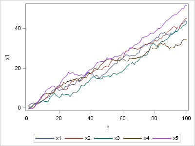
A Simulation and Visualization of Five Random Walks
As I have described previously, you can use the RANDGEN subroutine in SAS/IML software to generate the steps of the random walk. The following statements generate the steps for five random walks: each column of the x matrix represents a single random walk.
proc iml; NumWalks = 5; NumSteps = 100; Mean = 0.4; SD = 0.7; /** generate steps from N(Mean, SD) **/ /** each column is a different walk **/ x = j(NumSteps, NumWalks); call randseed(1234); call randgen(x, "Normal", Mean, SD); |
The position of the walker after each step is given by the cumulative sum of the step lengths, which you can compute by using the CUSUM function. To save memory, you can re-use the x matrix to store the positions:
do i = 1 to NumWalks; x[,i] = cusum(x[,i]); end; |
You can visualize the random walks by plotting the position as a function of the time, n.

Estimating the Likely Position after 100 Steps
If you want to estimate the likely position of the walker after 100 steps, you can simulate many random walks and look at the distribution of the final positions at n=100. For example, you can set NumWalks = 1000 in the previous program and re-generate the random walks. The final positions are obtained by the following statement:
/** positions after 100 steps **/ /** transpose into column vector **/ W100 = T(x[NumSteps,]); |
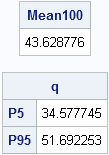
You can compute statistics of the simulated positions in order to estimate the expected location and the uncertainty in the estimate. The following statements estimate the likely location (which is 40 units) by using the MEAN function and a 90% confidence interval for the location by using the QNTL subroutine. (If you have not upgraded to SAS/IML 9.22, you can use the mean subscript reduction operator (W100[:]) and the QNTL module.)
Mean100 = mean(W100);
call qntl(q, W100, {0.05 0.95});
print Mean100, q[rowname={P5 P95}]; |

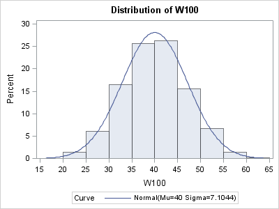
A histogram of the positions after 100 steps is shown below. The simulation indicates that the walker is expected to be 40 units from the origin after 100 steps. About 90% of the time, the final position of the walker is between 28 and 52 units.


3 Comments
Here is how to simulate a Weiner proces in SAS:
proc iml;
/* Simulate from a discrete Weiner process in SAS
See
"An Algorithmic Introduction to Numerical Simulation of
Stochastic Differential Equations" by D.J. Higham,
SIAM Review 43:525-546, 2001.
http://epubs.siam.org/doi/abs/10.1137/S0036144500378302
*/
proc iml;
call randseed(12345);
/* simulate N time steps from Weiner process on interval [0,Tf] */
N = 1000;
Tf = 5;
/* algorithm: step sizes are normally distributed */
N = N-1; /* X(0)=0, so N-1 random values */
dt = Tf/N; /* discretize problem */
sd = sqrt(dt); /* step length is ~ N(0, sd)*/
steps = randfun(N, "Normal", 0, sd); /* random step sizes */
x = 0 // cusum(steps); /* create path with X(0)=0 */
t = do(0, Tf, dt);
call series(t, x);
For a constant step size, this is called the "Drunkard's Walk." See "Simulating a drunkard's walk in SAS."
Pingback: Simulating a drunkard's walk in SAS - The DO Loop