Last week I generated two kinds of random point patterns: one from the uniform distribution on a two-dimensional rectangle, the other by jittering a regular grid by a small amount.

My show choir director liked the second method (jittering) better because of the way it looks on stage: there are no gaps and no two performers are too close to each other. The statistician in me wants to know what statistical properties make the jittered pattern more desirable than the other. Said differently, can I do any of the following?

• Compute a statistical measure that characterizes each kind of point pattern?
• Use statistics to predict whether a given pattern would be acceptable to her?

As part of my plan to learn new statistics, I've been reading Statistical Analysis and Modelling of Spatial Point Patterns by J. Illian, A. Penttinen, H. Stoyan, and D. Stoyan. The spatial statistics in this blog post come from their book.

This post has four parts:

1. I describe a simple test that indicates whether a point pattern is likely to have been generated from a random uniform distribution.
2. I implement the test in the SAS/IML language.
3. I simulate data to show what the test means and how it works.
4. I return to the above questions and show that the answer to both questions is "yes."

Complete Spatial Randomness --- A Test

Not all random configurations are created equal. A jittered pattern is random, but a pattern that is generated from a uniform distribution on a 2D rectangle exhibits complete spatial randomness (CSR).

There are several ways to test for CSR. Probably the easiest method is called the method of quadrats. The method consists of the following steps:

1. Divide the rectangular domain into k disjoint cells (bins) of equal area and count the number of points, c_i, that fall into each cell. You can use the Bin2D module for this step.
2. If the points were generated from a distribution with a uniform density, you would expect e = N/k points in each bin, where N is the total number of points. Subtract that value from the actual bin count to obtain the residual count for each bin.
3. Just as for two-way frequency tables, you can compute a normalized sum of the squared residuals and use that measure to determine whether the point pattern was likely to have come from a distribution with a uniform density. The computation is just the usual Pearson chi-square statistic: Σ (c_i - e)² / e.

The theory says that if a point pattern is generated from a uniform distribution, the Pearson statistic has an approximate chi-square distribution with k-1 degrees of freedom, provided that k > 6 and e > 1.

Ugh! It takes longer to explain the algorithm in words than it does to implement it in the SAS/IML language! It's time for a concrete example.

SAS/IML Code to Test for Complete Spatial Randomness

The following SAS/IML statements generate 20 points from a random uniform distribution, define a 3x3 grid on the unit square, and call the Bin2D module to count how many points are in each cell of the grid:

proc iml;
N = 20;
pUnif = j(N,2);
call randseed(1234);
call randgen(pUnif, "uniform"); /** generate random uniform **/
 
/** Define regular grid: 0, 0.33, 0.67, 1 **/
XMin = 0; XMax = 1; Nx = 3; dx = 1/Nx; 
YMin = 0; YMax = 1; Ny = 3; dy = 1/Ny;
XDiv = do(XMin, XMax, dx); 
YDiv = do(YMin, YMax, dy);
 
/** count the points in each cell **/
load module=Bin2D;
countUnif = Bin2D(pUnif, XDiv, YDiv);

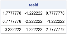
For this example, there are 20 points and 9 cells, so you should expect 2.22 points in each cell. The following statements compute the residuals (observed counts minus the expected value) for each cell and compute the Pearson statistic, which in spatial statistics is also known as the index of dispersion:

c = countUnif;
NBins = (ncol(XDiv)-1) * (ncol(YDiv)-1);
e = N/NBins;  /** expected value **/
resid = (c - e);
d = sum( resid##2 ) / e; /** index of dispersion **/
print resid;

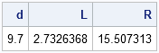
When the points come from a uniform random distribution, d has a 90% chance of being within the interval [L, R], where L and R are the following quantiles of the chi-square distribution:

L = quantile("chisquare", 0.05, NBins-1);
R = quantile("chisquare", 0.95, NBins-1);
print d L R;

What Does It Mean? Time to Simulate

My brain is starting to hurt. What does this all mean in practice?

What it means is that I can do the following experiment: simulate 1,000 point patterns from the random uniform distribution and compute the corresponding 1,000 Pearson statistics. If I plot a histogram of the 1,000 Pearson statistics, I should see that histogram looks similar to a chi-square distribution with 8 degrees of freedom and that roughly 100 (10%) of the Pearson statistics will be outside of the interval [L, R].

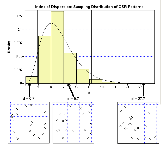
The adjacent image shows the results of the experiment, which I ran in SAS/IML Studio. The curve is a χ₈² distribution. The vertical lines are at the values L and R.

For this experiment, 71 point patterns have Pearson statistics that are outside of the interval. This is not quite 10%, but it is close. Repeating the experiment with different numbers of points (for example, N=30 or 50) and different grids (for example, a 2x3 or 4x3) results in similar histograms that also have roughly 10% of their values outside of the corresponding confidence interval.

The little scatter plots underneath give an example of a point pattern with the indicated Pearson statistic. The middle scatter plot (d=9.7) is the plot of the random points generated in the previous section. It is a "typical" point pattern from the random uniform distribution; most of the point patterns look like this one. You can see that there is a lot of variation in the cell counts for this configuration: one of the bins contains zero points, another contains five.

The scatter plot on the left (d=0.7) is a not a typical point pattern from the random uniform distribution. All of the cells in this pattern have two or three points. It is a little counterintuitive, but it is rare that a truly random uniform point pattern has points that are evenly spaced in the unit square.

The scatter plot on the right (d=27.7) shows the other extreme: more variation than is expected. Five of the cells in this pattern have zero or one points. A single cell contains almost half of the points!

What about the Jittered Patterns?

The previous graph implies that the arrangements of points that are randomly generated from a uniform distribution are rarely evenly spaced. The usual case exhibits gaps and clusters.

If you instead generate 1,000 jittered patterns, as in my previous post, the distribution of the Pearson statistics looks like the following image.

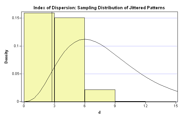
The distribution of Pearson's statistic does not follow a chi-square distribution for jittered patterns. Most of the values of Pearson's statistic are small, which makes sense because the statistic measures the departure from the average density, and the configurations are permutations of evenly spaced points.

It's time to revisit the questions posed at the beginning of this post.

Can I compute a statistical measure that characterizes each kind of point pattern? Yes. The Pearson statistic tends to be small for jittered point patterns and tends to be larger for random uniform configurations. However, if the Pearson statistic for an example pattern is, say, between 3 and 6, I can't predict whether the points were generated by using the jittering algorithm or whether they were generated from a random uniform distribution.

Can I use statistics to predict whether a given pattern might be acceptable to my director? Yes. Regardless of how the configuration was generated, a pattern that has a small value of the Pearson statistic (less than 3 for this example) does not exhibit gaps or clusters, and therefore will be acceptable to my director.

Although statistics can be used to check the appropriateness of certain blocking configurations, I don't think that my director will be replaced by a SAS/IML program anytime soon: she also plays the piano!