Many intervals in statistics have the form p ± δ, where p is a point estimate and δ is the radius (or half-width) of the interval. (For example, many two-sided confidence intervals have this form, where δ is proportional to the standard error.) Many years ago I wrote an article that mentioned that you can construct these intervals in the SAS/IML language by using a concatenation operator (|| or //). The concatenation creates a two-element vector, like this:

proc iml;
mu = 50; 
delta = 1.5;
CI = mu - delta  || mu + delta;   /* horizontal concatenation ==> 1x2 vector */

Last week it occurred to me that there is a simple trick that is even easier: use the fact that SAS/IML is a matrix-vector language to encode the "±" sign as a vector {-1, 1}. When SAS/IML sees a scalar multiplied by a vector, the result will be a vector:

CI = mu + {-1  1}*delta;         /* vector operation ==> 1x2 vector */
print CI;

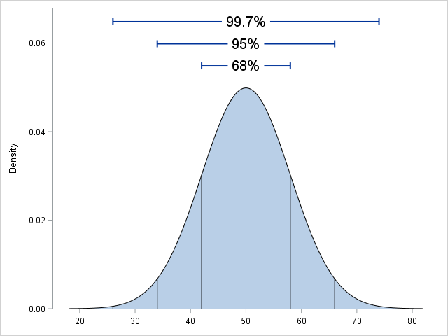You can extend this example to compute many intervals by using a single statement. For example, in elementary statistics we learn the "68-95-99.7 rule" for the normal distribution. The rule says that in a random sample drawn from a normal population, about 68% of the observations will be within 1 standard deviation of the mean, about 95% will be within 2 standard deviations, and about 99.7 % will be within 3 standard deviations of the mean. You can construct those intervals by using a "multiplier matrix" whose first row is {-1, +1}, whose second row is {-2, +2}, and whose third row is {-3, +3}. The following SAS/IML statements construct the three intervals for the 69-95-99.7 rule for a normal population with mean 50 and standard deviation 8:

mu = 50;  sigma = 8;
m = {-1 1,
     -2 2,
     -3 3};
 
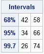
Intervals = mu + m*sigma;
ApproxPct = {"68%", "95%", "99.7"};
print Intervals[rowname=ApproxPct];

Just for fun, let's simulate a large sample from the normal population and empirically confirm the 68-95-99.7 rule. You can use the RANDFUN function to generate a random sample and use the BIN function to detect which observations are in each interval:

call randseed(12345);
n = 10000;                                /* sample size */
x = randfun(n, "Normal", mu, sigma);      /* simulate normal sample */
ObservedPct = j(3,1,0);
do i = 1 to 3;
   b = bin(x, Intervals[i,]);             /* b[i]=1 if x[i] in interval */
   ObservedPct[i] = sum(b) / n;           /* percentage of x in interval */
end;
 
results = Intervals || {0.68, 0.95, 0.997} || ObservedPct;
print results[colname={"Lower" "Upper" "Predicted" "Observed"}
              label="Probability of Normal Variate in Intervals: X ~ N(50, 8)"];

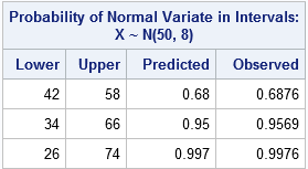
The simulation confirms the 68-95-99.7 rule. Remember that the rule is a mnemonic device. You can compute the exact probabilities by using the CDF function. In SAS/IML, the exact computation is p = cdf("Normal", m[,2]) - cdf("Normal", m[,1]);

In summary, the SAS/IML language provides an easy syntax to construct intervals that are symmetric about a central value. You can use a vector such as {-1, 1} to construct an interval of the form p ± δ, or you can use a k x 2 matrix to construct k symmetric intervals.