Rotation matrices are used in computer graphics and in statistical analyses. A rotation matrix is especially easy to implement in a matrix language such as the SAS Interactive Matrix Language (SAS/IML). This article shows how to implement three-dimensional rotation matrices and use them to rotate a 3-D point cloud.

Define a 3-D rotation matrix

In three dimensions there are three canonical rotation matrices:

• The matrix R_x(α) rotates points counterclockwise by the angle α about the X axis. Equivalently, the rotation occurs in the (y, z) plane.
• The matrix R_y(α) rotates points counterclockwise by the angle α in the (x, z) plane.
• The matrix R_z(α) rotates points counterclockwise by the angle α in the (x, y) plane.

Each of the following SAS/IML functions return a rotation matrix. The RotPlane function takes an angle and a pair of integers. It returns the rotation matrix that corresponds to a counterclockwise rotation in the (x_i, x_j) plane. The Rot3D function has a simpler calling syntax. You specify and axis (X, Y, or Z) to get a rotation matrix in the plane that is perpendicular to the specified axis:

proc iml;
/* Rotate a vector by a counterclockwise angle in a coordinate plane. 
        [ 1    0       0   ]
   Rx = [ 0  cos(a) -sin(a)]        ==> Rotate in the (y,z)-plane
        [ 0  sin(a)  cos(a)]
 
        [ cos(a)  0   -sin(a)]
   Ry = [   0     1      0   ]      ==> Rotate in the (x,z)-plane
        [ sin(a)  0    cos(a)]
 
        [ cos(a) -sin(a) 0]
   Rz = [ sin(a)  cos(a) 0]         ==> Rotate in the (x,y)-plane
        [   0       0    1]
*/
start RotPlane(a, i, j);
   R = I(3);  
   c = cos(a); s = sin(a);
   R[i,i] = c;  R[i,j] = -s;
   R[j,i] = s;  R[j,j] =  c;
   return R;
finish;
 
start Rot3D(a, axis);   /* rotation in plane perpendicular to axis */
   if upcase(axis)="X" then       
      return RotPlane(a, 2, 3);
   else if upcase(axis)="Y" then
      return RotPlane(a, 1, 3);
   else if upcase(axis)="Z" then
      return RotPlane(a, 1, 2);
   else return I(3);
finish;
store module=(RotPlane Rot3D);
quit;

NOTE: Some sources define rotation matrices by leaving the object still and rotating a camera (or observer). This is mathematically equivalent to rotating the object in the opposite direction, so if you prefer a camera-based rotation matrix, use the definitions above but specify the angle -α. Note also that some authors change the sign for the R_y matrix; the sign depends whether you are rotating about the positive or negative Y axis.

Applying rotations to data

Every rotation is a composition of rotations in coordinate planes. You can compute a composition by using matrix multiplication. Let's see how rotations work by defining and rotating some 3-D data. The following SAS DATA step defines a point at the origin and 10 points along a unit vector in each coordinate direction:

data MyData;               /* define points on coordinate axes */
x = 0; y = 0; z = 0; Axis="O"; output;    /* origin */
Axis = "X";
do x = 0.1 to 1 by 0.1;    /* points along unit vector in x direction */
   output;
end;
x = 0; Axis = "Y";
do y = 0.1 to 1 by 0.1;    /* points along unit vector in y direction */
   output;
end;
y = 0; Axis = "Z";
do z = 0.1 to 1 by 0.1;    /* points along unit vector in z direction */
   output;
end;
run;
 
proc sgscatter data=Mydata;
matrix X Y Z;
run;

If you use PROC SGSCATTER to visualize the data, the results (not shown) are not very enlightening. Because the data are aligned with the coordinate directions, the projection of the 3-D data onto the coordinate planes always projects 10 points onto the origin. The projected data does not look very three-dimensional.

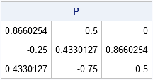
However, you can slightly rotate the data to obtain nondegenerate projections onto the coordinate planes. The following computations form a matrix P which represents a rotation of the data by -π/6 in one coordinate plane followed by a rotation by -π/3 in another coordinate plane:

proc iml;
/* choose any 3D projection matrix as product of rotations */
load module=Rot3D;
pi = constant('pi');
Rz = Rot3D(-pi/6, "Z");    /* rotation matrix for (x,y) plane */
Rx = Rot3D(-pi/3, "X");    /* rotation matrix for (y,z) plane */ 
Ry = Rot3D(    0, "Y");    /* rotation matrix for (x,z) plane */
P = Rx*Ry*Rz;              /* cumulative rotation */
print P;

For a column vector, v, the rotated vector is P*v. However, the data in the SAS data set is in row vectors, so use the transposed matrix to rotate all observations with a single multiplication, as follows:

use MyData;
read all var {x y z} into M;
read all var "Axis";
close;
RDat = M * P`;                    /* rotated data */

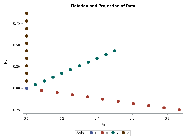
Yes, that's it. That one line rotates the entire set of 3-D data. You can confirm the rotation by plotting the projection of the data onto the first two coordinates:

title "Rotation and Projection of Data";
Px = RDat[,1]; Py = RDat[,2]; 
call scatter(Px, Py) group=Axis 
   option="markerattrs=(size=12 symbol=CircleFilled)";

Alternatively, you can write the rotated data to a SAS data set. You can add reference axes to the plot if you write the columns of the P` matrix to the same SAS data set. The columns are the rotated unit vectors in the coordinate directions, so using the VECTOR statement to plot those coordinates adds reference axes:

create RotData from RDat[colname={"Px" "Py" "Pz"}];
append from RDat;
close;
 
A = P`;          /* rotation of X, Y, and Z unit vectors */
create Axes from A[colname={"Ax" "Ay" "Az"}];  append from A; close;
Labels = "X":"Z";
create AxisLabels var "Labels";  append; close;
QUIT;
 
data RotData;    /* merge all data sets */
merge MyData Rot Axes AxisLabels;
run;
 
proc sgplot data=RotData;
   vector x=Ax y=Ay / lineattrs=(thickness=3) datalabel=Labels;
   scatter x=Px y=Py / group=Axis markerattrs=(size=12 symbol=CircleFilled);
   xaxis offsetmax=0.1; yaxis offsetmax=0.1; 
run;

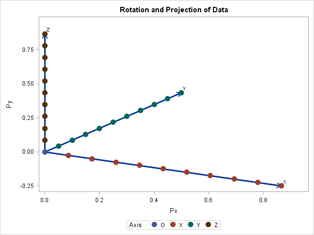
All the data points are visible in this projection of the (rotated) data onto a plane. The use of the VECTOR statement to add coordinate axes is not necessary, but I think it's a nice touch.

Visualizing clouds of 3-D data

This article is about rotation matrices, and I showed how to use matrices to rotate a 3-D cloud of observations. However, I don't want to give the impression that you have to use matrix operations to plot 3-D data! SAS has several "automatic" 3-D visualization methods that more convenient and do not require that you program rotation matrices. The visualization methods include

• The G3D procedure in SAS/GRAPH software creates 3-d scatter plots.
• The SAS/IML Studio application, which is part of SAS/IML software, supports a point-and-click interface to create rotating scatter plots, and you can also use the RotatingPlot class to create a 3-d scatter plot programmatically.

I also want to mention that Sanjay Matange created a 3-D scatter plot macro that uses ODS graphics to visualize a 3-D point cloud. Sanjay also uses rotation matrices, but because he uses the DATA step and PROC FCMP, his implementation is longer and less intuitive than the equivalent operations in the SAS/IML matrix language. In his blog he says that his macro "is provided for illustration purposes."

In summary, the SAS/IML language makes it convenient to define and use rotation matrices. An application is rotating a 3-D cloud of points. In my next blog post I will present a more interesting visualization example.