The SAS/IML language is used for many kinds of computations, but three important numerical tasks are integration, optimization, and root finding. Recently a SAS customer asked for help with a problem that involved all three tasks. The customer had an objective function that was defined in terms of an integral. The problem was to find the roots and the maximum value of the function.
An objective function that involves an integral
When constructing an example, it is always helpful to use a problem for which the exact answer is known. For this article, I will define the objective function as follows:
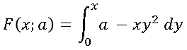
To make the example more realistic, I've included a parameter, a. For each value of x, this function requires evaluating a definite integral. (Integrals with an upper limit of x arise when integrating probability density functions.) The integrand is the function a – x y2. The dummy variable is y, so a and x are both treated as constant parameters when evaluating the integrand. Here are some useful facts about this function:
- The integrand is a polynomial in y, so the integral can be evaluated explicitly. The simplified expression for F is F(x; a) = ax – x4/3.
- The two real roots of F can be found explicitly. They are 0 and the cube root of 3a.
- The maximum value of F can be found explicitly. It is the cube root of 3a/4.
The remainder of this article demonstrates how to find the roots and maximum value of this function, which is defined in terms of an integral.
Defining the function in the SAS/IML language
When evaluating the integral, the values of x and a are constant. In order to integrate a function by using the QUAD subroutine, the module that defines the integrand must have exactly one argument, which supplies a value for the dummy variable, y. Consequently, list other parameters in the GLOBAL statement of the SAS/IML module that defines the integrand, as follows:
proc iml; /* Define the integrand, which will be called by QUAD subroutine. The integrand is a function of ONE variable: the "dummy" variable y. All other parameters are listed in the GLOBAL clause. */ start Integrand(y) global(a, x); return( a - x # y##2 ); finish; |
You can now define a SAS/IML module that evaluates the function F. I like to use param as the name of the argument to an objective function. The name helps me to remember that param is going to be manipulated by root-finding or nonlinear programming (NLP) algorithms in order to find the roots and extrema of the function. Here's how I would define the objective function that evaluates F:
/* Define a SAS/IML function that computes an integral. This module will be called by a root-finding or NLP routine. */ start ObjFunc(param) global(a, x); x = param; /* copy to global symbol */ limits = 0 || x; /* limits of integration: [0,x] */ call quad(w, "Integrand", limits); return( choose(x>=0, w, -w) ); /* trick to handle x<0 */ finish; |
I used a few tricks and techniques to define this module:
- The only argument to the function is param. This is the quantity that will be used to search for roots and extrema. It corresponds to the x in the mathematical expression F(x; a).
- The argument to the module cannot be named x because I have reserved that name for the global variable that is used by the INTEGRAND module. The SAS/IML syntax does not permit you to use the same name in the argument list and in the GLOBAL list for the same module. Instead, the OBJFUNC module copies the value of param to the x variable to ensure that the global variable remains in synch.
- For this function, the argument determines the limits of integration. If x is always positive, you don't need to do anything special. However, if you want to permit negative values for x, then you need to use the programming trick in my article about how to evaluate an integral where the limits of integration are reversed.
Visualize the function
When tasked with finding the roots or extrema of a function, I recommend that you visualize the function. This is useful for estimating the number of roots, the location of roots, and finding an initial guess for the optimum. Although visualization can be difficult when the objective function depends on a large number of variables, in this case the visualization requires merely graphing the function.
To draw the graph, you must specify values for any parameters. I will set a = 4/3. For that value of a, the function F has roots at 0 and the cube root of 4 (≈ 1.5874). The maximum of F occurs at x = 1.
/* visualize the objective function */
a = 4/3;
t = do(-1, 2, 0.05);          /* graph the function on [-1, 2] */
F = j(1, ncol(t));
do i = 1 to ncol(t);
   F[i] = ObjFunc(t[i]);      /* evaluate the objective function at each x */
end;
title "Objective Function for a = 4/3";
call Series(t, F) grid={x y} label={"x" "F(x)"}
other="refline 0 / axis=y"; /* add reference line at y=0 */ |
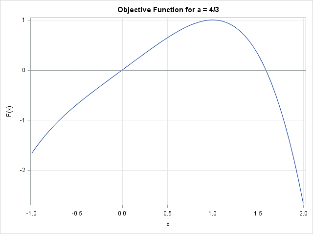
The graph indicates that the function has two roots, one near x=0 and the other near x=1.6. The function appears to have one maximum, which is located near x=1. Of course, these values depend on the value of the parameter a.
Graphing the function is a "sanity check" that gives us confidence that there are no mistakes in the definition of the objective function. It is very important to test and debug the module that defines the objective function before you try to find a maximum! Many people post programs to the SAS/IML Support Community and report that "the optimization reports a strange error." Sometimes they ask whether there is a problem with the SAS/IML optimizing routine. To paraphrase Shakespeare, usually the fault lies not in our optimizers, but in our objective function. Always verify that the objective function is defined correctly before you call an NLP routine.
Find roots of the function
The objective function is ready to work with. The following statements use the FROOT function to find roots on the interval [–1, 1] and [1, 2]:
/* find roots on [-1, 1] and [1, 2] */
intervals = {-1 1,
              1 2};
roots = froot("ObjFunc", intervals);    /* SAS/IML 12.1 */
print roots[format=6.4]; |
As stated earlier, the roots are at 0 and the cube root of 4 (≈ 1.5874).
Find a maximum of the function
To find the maximum, you can use one of the nonlinear programming functions in SAS/IML. In previous optimization problems I have used the NLPNRA subroutine, which uses the Newton-Raphson method to compute a maximum. However, Newton-Raphson is probably not the best choice for this problem because the function evaluation requires computing an integral, and therefore contains a small amount of numerical error. Furthermore, unless I "cheat" and use the exact solution to compute exact derivatives, the Newton-Raphson algorithm would have to use finite difference approximations to compute the derivative and second derivative at each point. For this problem these finite-difference computations are likely to be expensive and not very accurate.
Instead, I will use the Nelder-Mead simplex method, which in implemented in the NLPNMS subroutine. The simplex method solves an optimization problem without using any derivatives. This method can be a good choice for optimizing functions that have low precision, such as the result of evaluating an integral or the result of a simulation.
x0  = 0.5;      /* initial guess for maximum */
opt = {1,       /* find maximum of function  */
       0};      /* no printing */
call nlpnms(rc, Optimum, "ObjFunc", x0, opt); /* find maximum */
print Optimum[format=6.4]; |
As discussed previously, the maximum occurs at x=1.
This article has shown how to define a SAS/IML module that computes an integral in order to evaluate the function. The tips and techniques in this article should enable you to find the roots and extrema of complicated functions that arise in computational statistics.

1 Comment
Pingback: Guiding numerical integration: The PEAK= option in the SAS/IML QUAD subroutine - The DO Loop