There are a lot of useful probability distributions that are not featured in standard statistical textbooks. Some of them have distinctive names. In the past year I have had contact with SAS customers who use the Tweedie distribution, the slash distribution, and the PERT distribution. Often these distributions are used as part of a simulation study. This article describes how to simulate from the PERT distribution in SAS.
I had never heard of the PERT distribution prior to last week, but apparently it is related to the Project Evaluation and Review Technique (PERT), which is "a statistical technique for measuring and forecasting progress in research and development programs." Suppose management wants to know how long a project will take. This might be hard to estimate if the project consists of several interrelated tasks. However, perhaps you can estimate the length of each task and use those estimates to estimate the duration of the full project, hopefully with a statistical confidence interval.
To estimate the length of a task, you ask the manager (or some other expert) to tell you the minimum time it will take, the maximum time it will take, and the most likely time to complete the task. You might get an answer such as, "It will take at least five weeks, but probably more like eight weeks. Even in the worst case scenario, it'll be done in 20 weeks."
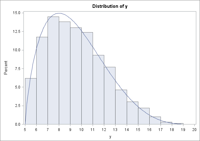
The PERT distribution turns those three numbers into a probability distribution, as shown in the following image. The minimum value of the distribution is 5, the maximum value is 20, and the mode of the distribution (the location of the peak) is at 8.
The PERT distribution isn't really a new distribution; it is a translated and scaled version of the well known beta distribution. The beta distribution is defined on the interval [0,1], but a simple linear transformation scales and translates the distribution onto any interval [min, max]. The beta distribution has two parameters, α and β, which determine the shape of the distribution. If I tell you that I want a beta distribution with a certain mean and a certain mode, you can find the values of α and β that satisfy my request. The mode is one of the parameters that the expert provides. The PERT distribution specifies that the mean is a certain weighted sum of the minimum, maximum, and mode.
Consequently, it is easy to simulate from the PERT distribution:
- Specify the parameters min, mode, and max. These are used to determine the mean of the distribution.
- Apply a linear transformation to determine the corresponding mode and mean for the beta distribution on [0,1]. Solve for the corresponding parameters, α and β.
- Simulate data from the Beta(α, β) distribution. Translate and scale the data onto the interval [min, max].
The following DATA step simulates 2,000 observations from a PERT distribution with min=5, mode=8, and max=20. The UNIVARIATE procedure is used to plot the resulting histogram and to overlay the underlying beta distribution:
data PERT; keep y; call streaminit(123); N = 2000; a = 5; /* min */ b = 8; /* mode */ c = 20; /* max */ mu = (a + 4*b + c)/6; /* mean as weighted sum of parameters */ /* find parameters for Beta distribution on [0,1] */ alpha = (mu-a)*(2*b-a-c)/((b-mu)*(c-a)); beta = alpha*(c-mu)/(mu-a); do i = 1 to N; y = rand("Beta", alpha, beta); /* y in [0,1] */ y = a + (c-a)*y; /* translate to [min, max] */ output; end; run; /* display histogram and fit to translated and scaled Beta */ proc univariate data=PERT; histogram y / beta(theta=5 sigma=15 alpha=1.8 beta=4.2) endpoints=(5 to 20); run; |
The graph (shown earlier in this article) shows the probability distribution of the duration of the task. Suppose that there are three sequential tasks, A, B, and C. Task A must be completed before B can begin, and Task B must be completed before C can begin. You can simulate the distribution of project duration times by simulating a time for each task and adding the three times together. Do this many times and you have an approximate distribution for the duration of the project.
The same process provides confidence intervals and probabilities for the duration of the project. For example, in the single-task case of the PERT distribution, you can estimate the probability that the task will take 12 weeks or longer:
data Prob; set PERT; Delay = (y>12); /* indicator var: 1 if task takes more than 12 weeks */ run; proc freq data=Prob; table Delay / nocum; /* what percent of times took more than 12 weeks? */ run; |
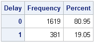
For this one task, the probability that it will take more than 12 weeks is 19%. In the case of a single task, you can use the QUANTILE function to compute probabilities from the beta distribution, but in general the project time is the sum of several beta random variables, each with different parameters, so you need to use the simulated sampling distribution to estimate the probability.
I can see how techniques like this would be very useful for keeping track of big projects. Apparently this technique was used in the 1960's for estimating the length of projects in the US Navy and for projects leading up to the 1968 (Grenoble) Olympics.

10 Comments
Great story. In case you have any readers who are JMP users and want to take a sample from the PERT distribution, I wrote this script to mimic your SAS program.
Hunh. I thought PERT used the triangular distribution. You learn something new every day.
Hi Rick,
PERT has another param, lambda. The λ (lambda) parameter controls the scale of the distribution (the peakedness).
Is possible adding λ in your procedure?
tnx
N
You didn't supply a reference, but I suspect you want something like these two statements:
This formula doesn't work when 2*b-a-c = 0
e.g.
Yes. If 2*b-a-c=0 then alpha=beta=0 and the beta distribution is degenerate. If you click on the link the "the PERT distribution" in the first paragraph, you will find an article that describes limitations of the PERT distribution. Included in that article is a generalization of the PERT distribution that can eliminate some of the degeneracies. See also the comment just prior to yours.
Please help explain the statements below:
alpha = (mu-a)*(2*b-a-c)/((b-mu)*(c-a));
beta = alpha*(c-mu)/(mu-a);
what's the origin of these statements?
Please re-read the first six paragraphs. If an expert gives you an estimate of the minimum time (a), the most likely time (b), and the maximum time (c), you can use the previous formulas to compute the parameters (alpha and beta) for a probability distribution that models the time as a random variable. The probability distribution is called the beta distribution. The (alpha, beta) values are the ones that make the beta distribution have a minimum at 'a', a mode at 'b', and a maximum at 'c'.
Thank you quite much for your patience!! What confuses me is actually the procedure leading to alpha's formula using estimate of minimum time(a),the most likely time(b) and the maximum time(c).
I have learnt another literature ——Teaching Project Simulation in Excel using PERT-Beta Distributions, written by Ron Davis, which gives complete formula for a Beta distribution defined on the interval [a,b] with parameters [Alpha,Beta,a,b].It has MEAN: mu = a + (b-a)*(Alpha/(Alpha+Beta) ;VARIANCE:(Alpha/(Alpha+Beta))*(Beta/(Alpha+Beta))*((b-a)2/(Alpha+Beta+1)).
However, I failed to derive "alpha = (mu-a)*(2*b-a-c)/((b-mu)*(c-a));" according to the formula above. Can you help me?
The computer code shows the formulas. It is easier if you work with the standard beta distribution on [0,1], then linearly scale it to get the beta distribution on [a,b]. For the beta distribution on [0,1], the mode is at (Alpha-1)/(Alpha+Beta-2). Unfortunately, I don't have time to show you how to derive the formulas. Good luck.