I've blogged several times about multivariate normality, including how to generate random values from a multivariate normal distribution. But given a set of multivariate data, how can you determine if it is likely to have come from a multivariate normal distribution?
The answer, of course, is to run a goodness-of-fit (GOF) test to compare properties of the data with theoretical properties of the multivariate normal (MVN) distribution. For univariate data, I've written about the usefulness of the quantile-quantile (Q-Q) plot to model the distribution of data, and it turns out that there is a similar plot that you can use to assess multivariate normality. There are also analytic GOF tests that can be used.
To see how these methods work in SAS, we need data. Use the RANDNORMAL function in SAS/IML software to generate data that DOES come from a MVN distribution, and use any data that appears nonnormal to examine the alternative case. For this article, I'll simulate data that is uniformly distributed in each variable to serve as data that is obviously not normal. The following SAS/IML program simulates the data:
proc iml;
N = 100; /* 100 obs for each distribution */
call randseed(1234);

/* multivariate normal data */
mu = {1 2 3};
Sigma = {9 1 2,
       1 6 0,
       2 0 4 };
X = randnormal(N, mu, Sigma);

/* multivariate uniform data */
v = j(N, ncol(mu));         /* allocate Nx3 matrix*/
call randgen(v, "Uniform"); /* each var is U[0,1] */
v = sqrt(12)*(v - 1/2);     /* scale to mean 0 and unit variance */
U = mu + T(sqrt(vecdiag(Sigma))) # v; /* same mean and var as X */ |
A graphical test of multivariate normality
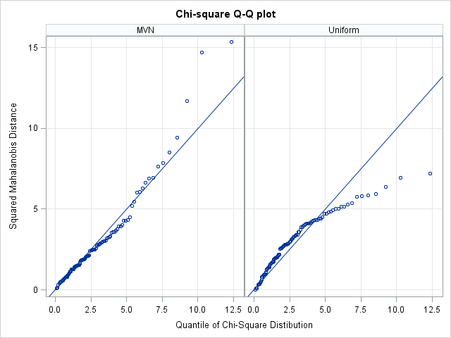
If you want a quick check to determine whether data "looks like" it came from a MVN distribution, create a plot of the squared Mahalanobis distances versus quantiles of the chi-square distribution with p degrees of freedom, where p is the number of variables in the data. (For our data, p=3.) As I mentioned in the article on detecting outliers in multivariate data, the squared Mahalanobis distance has an approximate chi-squared distribution when the data are MVN. See the article "What is Mahalanobis distance?" for an explanation of Mahalanobis distance and its geometric interpretation.
I will use a SAS/IML function that computes Mahalanobis distances. You can insert the function definition into the program, or you can load the module from a SAS catalog if it was previously stored. The following program computes the Mahalanobis distance between the rows of X and the sample mean:
load module=Mahalanobis; /* or insert module definition here */ Mean = mean(X); /* compute sample mean and covariance */ Cov = cov(X); md = mahalanobis(X, Mean, Cov); |
For MVN data, the square of the Mahalanobis distance is asymptotically distributed as a chi-square with three degrees of freedom. (Note: for a large number of variables you need a very large sample size before the asymptotic chi-square behavior becomes evident.) To plot these quantities against each other, I use the same formula that PROC UNIVARIATE uses to construct its Q-Q plots, as follows:
md2 = md##2;
call sort(md2, 1);
s = (T(1:N) - 0.375) / (N + 0.25);
chisqQuant = quantile("ChiSquare", s, ncol(X)); |
If you plot md2 versus chiSqQuant, you get the graph on the left side of the following image. Because the points in the plot tend to fall along a straight line, the plot suggests that the data are distributed as MVN. In contrast, the plot on the right shows the same computations and plot for the uniformly distributed data. These points do not fall on a line, indicating that the data are probably not MVN. Because the samples contain a small number of points (100 for this example), you should not expect a "perfect fit" even if the data are truly distributed as MVN.
Goodness-of-fit tests for multivariate normality
Mardia's (1974) test multivariate normality is a popular GOF test for multivariate normality. Mardia (1970) proposed two tests that are based definitions of multivariate skewness and kurtosis. (See von Eye and Bogat (2004) for an overview of this and other methods.) It is easy to implement these tests in the SAS/IML language.
However, rather than do that, I want to point out that SAS provides the %MULTNORM macro that implements Mardia's tests. The macro also plots the squared Mahalanobis distances of the observations to the mean vector against quantiles of a chi-square distribution. (However, it uses the older GPLOT procedure instead of the newer SGPLOT procedure.) The macro requires either SAS/ETS software or SAS/IML software. The following statements define the macro and call it on the simulated MVN data:
/* write data from SAS/IML to SAS data set */ varNames = "x1":"x3"; create Normal from X[c=varNames]; append from X; close Normal; quit; /* Tests for MV normality */ %inc "C:\path of macro\multnorm.sas"; %multnorm(data=Normal, var=x1 x2 x3, plot=MULT); |
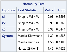
The macro generates several tables and graphs that are not shown here. The test results shown in the preceding table indicate that there is no reason to reject the hypothesis that the sample comes from a multivariate normal distribution. In addition to Mardia's test of skewness and kurtosis, the macro also performs univariate tests of normality on each variable and another test called the Henze-Zirkler test.
Another graphical tool: Plot of marginal distributions
To convince yourself that the simulated data are multivariate normal, it is a good idea to use the SGSCATTER procedure to create a plot of the univariate distribution for each variable and the bivariate distribution for each pair of variables. Alternatively, you can use the CORR procedure as is shown in the following statements. The CORR procedure can also produce the sample mean and sample covariance, but these tables are not shown here.
/* create scatter plot matrix of simulated data */ proc corr data=Normal COV plots(maxpoints=NONE)=matrix(histogram); var x:; ods select MatrixPlot; run; |
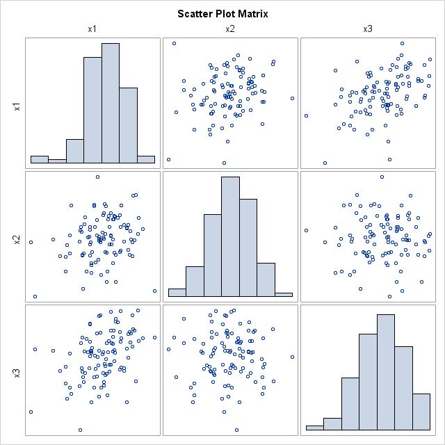
The scatter plot matrix shows (on the diagonal) that each variable is approximately normally distributed. The off-diagonal elements show that the pairwise distributions are bivariate normal. This is characteristic of multivariate normal data: all marginal distributions are also normal. (This explains why the %MULTNORM macro includes univariate tests of normality in its test results.) Consequently, the scatter plot matrix is a useful graphical tool for investigating multivariate normality.

17 Comments
Pingback: The curse of dimensionality: How to define outliers in high-dimensional data? - The DO Loop
Pingback: Popular! Articles that strike a chord with SAS users - The DO Loop
Dear sir
would you send syntax for Multivariate normality data test in SAS?
Thank you
bedasamoke@gmail.com
See the documentation of the %MULTNORM macro: http://support.sas.com/kb/24/983.html
Dear Rick Wicklin, thanks for the interesting post. Some questions from a newbie in statisics.
Outliers can affect the distribution of our data points (more precise, residuals) but an extreme value may belong to distribution's tail.
1) Do we have to calculate residuals to check for multivariate normality (MVN) as we do in a univariate case and submit them for the tests you mention here ?
2) Do we need to check MVN before testing for outliers or vice versa ?
3) Do the number of variables determine the number of dimensions (d) in MV normal distribution ?
Sincerely,
Stan
There is no regression problem here. We have a set of N observations and d variables. We want to check whether these data are likely to have come from a MVN distribution.
1) There is no response variable. The univariate analog is having N univariate data and asking whether a normal distribution fits the data. You can use PROC UNIVARIATE in the 1-D case.
2) If there is an extreme outlier in the data, that will affect the sample mean and covariance, and correspondingly affect the fit. If some data point is obviously wrong (for example, a coding error or a known abnormality), you might want to exclude it before fitting the MVN distribution.
3) Yes, the number of variables determines the dimension.
Dear Rick,
thanks for your reply. Another short question: does the sentence "There is no regression problem here." mean that we have to consider raw data rather than residuals for testing a (general/mixed) linear model assumptions in cases where the independent variable(s) is(are) categorical rather than continuous (like here: http://stats.stackexchange.com/q/11887)?
Thank you.
No, my statement meant "In this article, I do not assume that there is a regression problem." For your application, examine whether the residuals are (univariate) normal. In other words, if you want to test whether a linear model captures all of the "signal" and leaves you with residuals that are MVN, then you would test the residuals for normality. I like to use a Q-Q plot, rather than a formal hypothesis test.
Dear Rick Wicklin,
I want to know about probability density function that you use to generate multivariate uniform data?
In this article I generate random NORMAL data, and the first hyperlink provides more information about MVN data, or see the documentation for the RANDNORMAL function in SAS. To generate MV uniform data on [0,1]k, you can generate k independent random variables on [0,1].
Thank you for answer.
Dear Rick Wicklin,
What is the multivariate uniform distributuion p.d.f.? Could you please show me in an equation form?
Moreover, please let me know about your reference about this distribution p.d.f.. It would be very important part of my study.
Thank you in advance.
The pdf of a multivariate uniform distribution is the constant 1/V where V is the volume of the region. This follows from the definition of a probability density. For example, on the unit square [0,1] x [0,1], the pdf is f(x,y)=1. Notices that if you integrate the density over the region, you obtain 1, which is the total probability. Similarly, on the rectangle [a,b] x [c,d], the pdf is f(x,y)=(b-a)(d-c). A reference would be any introductory text on probability or measure theory.
another simple approach is to fit an intercept model in PROC MODEL to test bivariate (or multivariate) normality between X and Y or.....more variables.
proc model;
y=a;
x=b;
fit y x /normal;
Thanks for the comment. That is exactly the code that the %MULTNORM macro produces if you have a license for SAS/ETS. See the macro source and search for 'proc model'.
Dear Sr,
I paste your code and it doesn't work:
/* create scatter plot matrix of covid data */
proc corr data=Normal COV plots(maxpoints=NONE)=matrix(histogram);
var ratio_1, ratio_2;
ods select MatrixPlot;
run;
I am getting that output MatrixPlot was not created.
Make sure you are running with ODS graphics turned on. Put
ODS GRAPHICS ON;
prior to the PROC CORR step.