I've previously described ways to solve systems of linear equations, A*b = c. While discussing the relative merits of the solving a system for a particular right hand side versus solving for the inverse matrix, I made the assertion that it is faster to solve a particular system than it is to compute an inverse and use the inverse to solve the system.
In particular, in terms of the SAS/IML SOLVE function and INV function, I asserted that it is faster to run b = solve(A,c); than Ainv = inv(A); b = Ainv * c;.
A colleague asked a good question: "How much faster?"
The following SAS/IML program answers this question. The program generates a random n x n matrix for a range of values for n. For each matrix, the program times how long it takes to solve the linear system. The program is adapted from Chapter 15 of Wicklin (2010), Statistical Programming with SAS/IML Software.
proc iml;
/* this program computes the solution to a linear system in two
   different ways and compares the performance of each method */
size = T(do(100, 1000, 100)); /* 100, 200, ... 1000 */
results = j(nrow(size), 2);   /* allocate room for results */
do i = 1 to nrow(size);
   n = size[i];
   A = rannor(j(n,n,1));           /* n x n matrix */
   b = rannor(j(n,1,1));           /* n x 1 vector */

   /* use the INV function to solve a linear system Ax=b */
   t0 = time();                    /* begin timing INV */
      AInv = inv(A);               /* compute inverse of A */
      x = AInv*b;                  /* solve linear equation A*x=b */
   results[i,1] = time() - t0;     /* end timing */

   /* use the SOLVE function to solve the same linear system */
   t0 = time();                    /* begin timing SOLVE */
      x = solve(A,b);              /* solve linear equation directly */
   results[i,2] = time() - t0;     /* end timing */
end; |
You can save the times to a SAS data set and use the SGPLOT procedure to compare the performance of the two methods:
/* write results to a data set */
y = size || results;
create Performance from y[colname={"Size" "INV" "SOLVE"}];
append from y;
quit;

title "Time Required to Solve a Linear System: INV versus SOLVE";
title2 "From Wicklin (2010), Statistical Programming with SAS/IML Software";
proc sgplot data=Performance;
  series x=Size y=INV / curvelabel;
  series x=Size y=SOLVE /curvelabel;
  yaxis grid label="Time (s)";
  xaxis grid label="Size of Matrix";
run; |
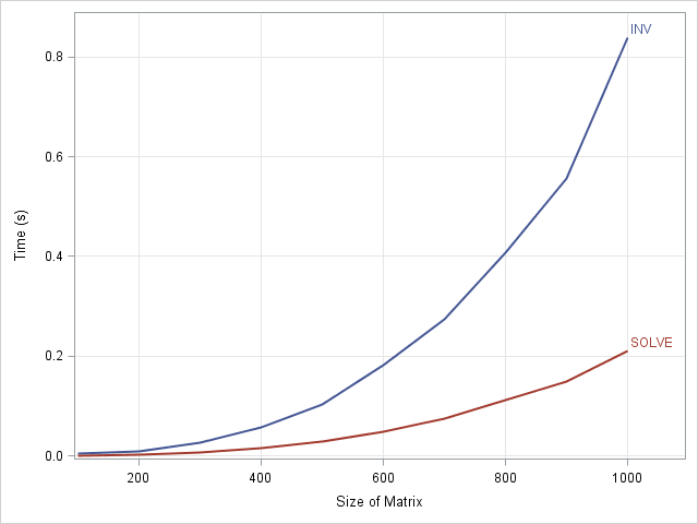
For a 1000 x 1000 matrix, it takes about 0.8 seconds to solve the system by computing the matrix inverse, whereas it takes 0.2 seconds to solve the system directly. That ratio is fairly typical: it takes about four times longer to solve a linear system with INV as with SOLVE.
This result is not unique to SAS/IML software. Although the algorithm that is used to compute each solution will affect the shape of the curves, solving a linear system directly should be faster than a solution that involves computing a matrix inverse.

16 Comments
Great benchmarking! I suppose that the responsable would be the computing cost to do all the inverse matrix. I would say almost exponentional increase time! Cool!
Thanks for the comment. You can show that the algorithms are O(n^3), which means that number of computations increases cubicly with the dimension of the n x n matrix. That's better than an exponential increase, but it still means that inverting a big matrix requires a lot of computations!
Hi, I'm new to SAS/ML and I have a few questions ...
How did you ensure that your randomly generated matrix actually has an inverse ? Did your code break at some point because of the generated matrix being singular (inv() function could return a generalized inverse though, but does it) ?
Thanks!
Welcome to SAS/IML, and thanks for the perceptive question! I actually considered discussing this issue, but decided it might distract from my main point. The answer is that I did not check that the randomly generated matrix has an inverse, I merely relied on probability. The set of (n x n) matrices is equivalent to Euclidean space with dimension n##2. It turns out that the set of singular (n x n) matrices has dimension (n##2 - 1) within that larger space. Therefore if you choose a matrix at random, you are going to choose a singular matrix with probability zero.
If I get "unlucky" and generate a singular matrix, my code will stop with an error, because I am not handling that case.
I agree with your conclusion, but I don't get the argument. "Dimension" usually refers to a linear space, but the set of singular matrices isn't a linear space. (Eg, [1,0;0,0] and [0,0;0,1] are singular matrices, but their sum isn't.) Does it mean something different here?
I'm not suggesting the probability of drawing a singular matrix is non-zero, I'm just not sure how you're getting there.
Yes, it can be confusing. As you say, the set of singular matrices is not a linear space. It is something called a "manifold" (or "surface," if that's easier to visualize) and is defined by the equation det(A)=0. The determinant equation constrains the singular matrices to be a dimension n##2 - 1 manifold inside of n##2 Euclidean space. An analogy is a curve in 2D space that satisfies a constraint such as x-y##2 = 0. That curve is not a linear space, but it is a 1D object inside of 2D space.
Thanks for the reply, I follow now. Although I've never thought about manifolds, your reply plus some thinking about how a singular matrix is 'restricted' made the intuition clear.
Pingback: What is the chance that a random matrix is singular? - The DO Loop
Pingback: Readers’ choice 2011: The DO Loop’s 10 most popular posts - The DO Loop
Pingback: Use the Cholesky transformation to correlate and uncorrelate variables - The DO Loop
Pingback: How to compute Mahalanobis distance in SAS - The DO Loop
Pingback: The power method: compute only the largest eigenvalue of a matrix - The DO Loop
Pingback: Eight tips to make your simulation run faster - The DO Loop
I think accuracy mav be different. Because the solution achieved by inverse has a high accuracy.
Generally speaking, the SOLVE function is numerically more stable (less likely to propogate errors) than the INV function. See, for example, the introduction to Du Croz and Higham (1992).
Pingback: 6 tips for timing the performance of algorithms - The DO Loop