In a previous blog post, I presented a short SAS/IML function module that implements the trapezoidal rule. The trapezoidal rule is a numerical integration scheme that gives the integral of a piecewise linear function that passes through a given set of points.
This article demonstrates an application of using the trapezoidal rule: computing the area under a receiver operator characteristic (ROC) curve.
ROC Curves
Many statisticians and SAS programmers who are familiar with logistic regression have seen receiver operator characteristic (ROC) curves. The ROC curve indicates how well you can discriminate between two groups by using a continuous variable. If the area under an ROC curve is close to 1, the model discriminates well; if the area is close to 0.5, the model is not any better than randomly guessing.
Let Y be the binary response variable that indicates the two groups. Let X be a continuous explanatory variable. In medical applications, for example, Y might indicate the presence of a disease and X might indicate the level of a certain chemical or hormone. For this blog post, I will use a more whimsical example. Let X indicate the number of shoes that a person has, and let Y indicate whether the person is female.
The following data indicate the results of a nonscientific survey of 15 friends and family members. Each person was asked to state approximately how many pairs of shoes (5, 10, ..., 30+) he or she owns. For each category, the data show the number of females in that category and the total number of people in that category:
data shoes; input Shoes Females N; datalines; 5 0 1 10 1 3 15 1 2 20 3 4 25 3 3 30 2 2 ; |
An easy way to generate an ROC curve for these data is to use the LOGISTIC procedure. You can get the actual values on the ROC curve by using the OUTROC= option on the MODEL statement:
ods graphics on; proc logistic data=shoes plots(only)=roc; ods select ROCcurve; model Females / N = shoes / outroc=roc; run; |
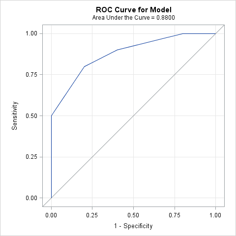
Notice that the graph has a subtitle that indicates the area under the ROC curve. If you want to check the result yourself, the points on the ROC curve are contained in the ROC data set:
proc print data=roc; var _1mSpec_ _Sensit_; run; |
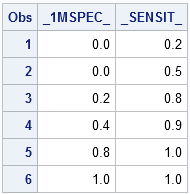
I used these points in my previous blog post. You can refer to that post to verify that, indeed, the area under the ROC curve is 0.88, as computed by the SAS/IML implementation of the trapezoidal rule.
By the way, the area under the ROC curve is closely related to another statistic: the Gini coefficient. Murphy Choy writes about computing the Gini coefficient in SAS in a recent issue of VIEWS News, a newsletter published by members of the international SAS programming community. The Gini coefficient is related to the area under the ROC curve (AUC) by the formula G = 2 * AUC – 1, so you can extend the program in my previous post to compute the Gini coefficient by using the following SAS/IML statement:
Gini = 2 * TrapIntegral(x,y) - 1; |
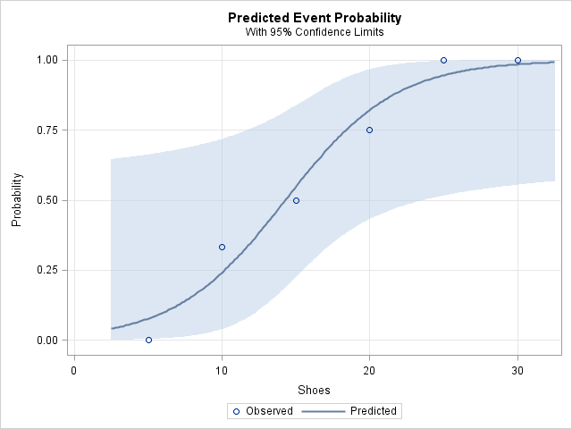
How well does the number of shoes predict gender in my small sample? The answer is "moderately well." The logistic model for these data predicts that a person who owns fewer than 15 pairs of shoes is more likely to be male than female. A person with more than 20 pairs of shoes is likely to be female. The area under the ROC curve (0.88) is fairly close to 1, which indicates that the model discriminates between males and females fairly well.
The logistic model is summarized by the following plot (created automatically by PROC LOGISTIC), which shows the predicted probability of being female, given the number of pairs of shoes owned. Notice the wide confidence limits that result from the small sample size.

9 Comments
Great post- I wish I had known you could access the ROC data set in SAS! I would have used that info in a recent presentation. I'm going to have to stay on top of your future posts. Thanks.
Pingback: The area under a density estimate curve - The DO Loop
Pingback: Computing an ROC Curve from Basic Principles - The DO Loop
Very Clear. My current problem is how to compare two different AUC- (two different diagosis procedure tests as continuous explanatory variables for the same Y as the presence of the disease).
Thank you for your answer.
PROC LOGISITC does this automatically. Use the ROC statement. The PROC LOGISTIC doc contains an example of comparing ROC curves.
I am trying to get a ROC curve (AUC) for model validation. I need to use the model with the intercept and beta coefficients from the original study. Is there a way to do this in SAS?
I don't know. Post this question to the Statistical Procedures Support Community. There are experts there that know more about logistic regression and ROC curves than I do. One idea: To test whether your model (with your data) has the same AUC as reported in the published study, you can use the ROC statement in PROC LOGISTIC to compute the area and confidence interval. If your CI contains the AUC reported by the study, they are statistically the same.
Pingback: The DIF function: Compute lagged differences and finite differences - The DO Loop
There seems to be confusion between the Gini Coefficent and the Accuracy Ratio within SAS as well as in the wider Statistical Community
One of the above two measures is defined in terms of the Area under the ROC Curve and the other is defined in terms of the Lorenz Cumulative Accuracy Profile Curve
The difference is significant because one measure can be used to compare two models from different samples while the other cannot be used for this purpose.
In a ( binary logistic regression model within Credit Risk ) context, the one measure is sensitive to the ratio of "Bads" to "Goods" while the other measure is robust with respect to this ratio.