In a previous article I discussed the situation where you have a sequence of (x,y) points and you want to find the area under the curve that is defined by those points. I pointed out that usually you need to use statistical modeling before it makes sense to compute the area.
However, there is a numerical technique that is very useful for a wide range of numerical integration scenarios, and that is the trapezoidal rule.
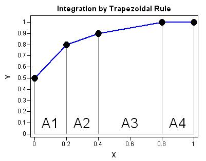
The following graph illustrates the trapezoidal rule. Given a set of points (x1, y1), (x2, y2), ..., (xn, yn), with x1 ≤ x2 ≤ ... ≤ xn, the trapezoidal rule computes the area of the piecewise linear curve that passes through the points. You can compute the area under the piecewise linear segments by summing the area of the trapezoids A1, A2, A3, and A4. (Sometimes a trapezoid is degenerate and is actually a rectangle or a triangle.)
Implementing the Trapezoidal Rule in SAS/IML Software
It is easy to use SAS/IML software (or the SAS DATA step) to implement the trapezoidal rule. The area of a trapezoid defined by (xi, yi) and (xi+1, yi+1) is
( xi+1 – xi ) ( yi + yi+1 ) / 2The first term is just the width of the subinterval [xi, xi+1] and the second term is the average of the heights at each end of the subinterval.
The following user-defined function computes the area under the piecewise linear segments that connect the points. The function does not check that the x values are sorted in nondecreasing order.
proc iml;
/**Given two vectors x,y where y=f(x), this module
   approximates the definite integral int_a^b f(x) dx
   by the trapezoid rule.
   The vector x is assumed to be in numerically increasing
   order so that a=x[1] and b=x[nrow(x)].
   The module does not assume equally spaced intervals.
   The formula is
   Integral = Sum(  (x[i+1] - x[i]) * (y[i] + y[i+1])/2 )
**/
start TrapIntegral(x,y);
   N = nrow(x);
   dx    =   x[2:N] - x[1:N-1];
   meanY = ( y[2:N] + y[1:N-1] )/2;
   return( dx` * meanY );
finish;

/** test it **/
x = {0.0, 0.2, 0.4, 0.8, 1.0};
y = {0.5, 0.8, 0.9, 1.0, 1.0};
area = TrapIntegral(x,y);
print area; |
Notice that the implementation does not require equally spaced points. The width of all subintervals are computed in a single statement and assigned to the vector dx. Similarly, the average of the heights are computed in a single statement and assigned to the vector meanY. The summation of all the areas is then computed by using a dot product of vectors. (Equivalently, the module could also return the quantity sum(dx # meanY), but the dot product is the more efficient computation.)
The simplicity of the trapezoidal rule makes it an ideal for many numerical integration tasks. Also, the trapezoidal rule is exact for piecewise linear curves such as an ROC curve. Also, as John D. Cook points out, there are other situations in which the trapezoidal rule performs more accurately than other, fancier, integration techniques.
The trapezoidal rule is not as accurate as Simpson's Rule when the underlying function is smooth, because Simpson's rule uses quadratic approximations instead of linear approximations. The formula is usually given in the case of an odd number of equally spaced points. Leave a comment to discuss the relative advantages and disadvantages of Simpson's rule as compared to the trapezoidal rule.
In a future blog post, I will use the TrapIntegral function to integrate some functions that arise in statistical data analysis.

17 Comments
Fantastic work! I applied it in my daily routine immediately. Thanks a lot.
Pingback: A statistical application of numerical integration: The area under an ROC curve - The DO Loop
Pingback: The area under a density estimate curve: Nonparametric estimates - The DO Loop
If you could state the strengths and limitations of both simpson's rule and trapezodial rule that would be greatly appreciated. However, the work already posted is great.
The strength of the trapezoidal rule is that it is fast and it is exact for piecewise linear functions. The strength of Simpson's rule is that it is usually more accurate: it has a smaller error when integrating smooth functions. The limitations for both algorithms is that they are designed for finite intervals. They are also require that you choose the number of subdivisions in advance, which is why I use the QUAD subroutine in SAS/IML software for serious work. The QUAD subroutine implements an adaptive Romberg-type algorithm that is is more accurate than Simposon's Rule and can work on infinite domains.
I need some help on the application of trapezoidal rule or simpson rule in mining metallurgy, where exactly can we apply these two rules?
These rules enable you to numerically approximate an integral. Integrals appear in many areas of material science, including loads, shears, stresses, torsion, etc. See any engineering or calculus textbook.
Pingback: An easy way to approximate a cumulative distribution function - The DO Loop
what about missing data points? what is the best way to estimate area under the curve if there is a missing data point?
Use the trapezoid rule applied to the nonmissing data, which is equivalent to linear interpolation of missing Y values.
So if I have two groups (placebo vs active) and 5 timepoints (i.e., 4 trapezoids) for a measurement scale. Several of the subjects are missing the last 1-2 timepoints. If I sum the values of the trapezoids to a final AUC for each subject, can I simply compare mean AUC's with a t-test (assuming normally distributed)?.
If so, some of the total AUCs will be much smaller because of missing values--how can I handle this post hoc?
If you want to compare two ROC curves, use the ROC and ROCCONTRAST statements in PROC LOGISTIC. If you have further questions, you can post them to the SAS Support Communities.
One of the objectives of pharmacokinetic studies is the determination of the area under the curve (AUC) parameter. The area under the curve represents the proportion of the drug absorbed into the systemic circulation and the time required to do so.
This pharmacokinetic parameter is used to determine the total exposure of a person to the drug over a period of time and is required by regulatory authorities to determine bioavailability and conclude bioequivalence or the absence of pharmacokinetic interactions.
The area under the curve can be obtained through two methodologies: the first involves nonlinear regression model analysis, or through non-compartmental analysis (NCA).
NCA is usually the preferred methodology as it requires fewer assumptions than model-based approaches. There are four methods to determine the AUC through non-compartmental analysis: Linear Log Trapezoidal, Linear Trapezoidal Interpolation, Linear Up Log Down, and Linear/Logarithmic Trapezoidal Interpolation.
The linear trapezoidal method uses linear interpolation between data points to calculate the AUC. This method is required by the OGD and the FDA, and it is the standard for bioequivalence trials.
The logarithmic trapezoidal method uses logarithmic interpolation between data points to calculate the AUC. This method is more accurate when concentrations are decreasing because drug elimination is exponential (making it linear on a logarithmic scale).
Below you will find a slide about your issue.
https://bebac.at/lectures/Moscow2012WS2.pdf
https://bebac.at/lectures/Moscow2012WS3.pdf
Hello,
Thanks for your explanation. How can I implement this code in to the Malab script?
I want to make a report in Trapezoid rule and simpson rule.
What the advantage and disadvantage for Trapezoid rule and simpson rule
What the theory of each one and their applications?
Thank you
Theoretically, each method is based on evenly dividing an interval into subintervals. The trapezoidal rule uses a linear approximation to the function on each interval, whereas Simpson's rule uses a quadratic approximation. The area under the (approximate) curve is computed for each subinterval, and the areas are summed to approximate the integral on the full interval. Because Simpson's rule uses a quadratic approximation on each subinterval, Simpson's rule is more accurate when each method uses the same number of subintervals. The advantage of the trapezoidal rule is that it is very fast and it is exact for piecewise linear functions.
can you please discuss the limitation of trapezoidal method