While at a conference recently, I was asked whether it was possible to use SAS to simulate data from an inverse gamma distribution. The SAS customer had looked at the documentation for the RAND function and did not see "inverse gamma" listed among the possible choices.

The answer is "yes." The distributions that are listed for the RAND function (and the RANDGEN subroutine in SAS/IML) are building blocks that enable you to build other less common distributions. I discuss this in Chapter 7 of Simulating Data with SAS where I show how to simulate data from a dozen distributions that are not directly supported by the RAND function.

When I want to simulate data from a distribution that is not directly supported by the RAND function, I first look at the documentation for the MCMC procedure, which lists the definitions for more than 30 distributions. If I can't find the distribution there, I walk to the library to browse the ultimate reference guide: the two volumes of Continuous Univariate Distributions by Johnson, Kotz, and Balakrishnan (2nd edition, 1994). The Wikipedia article on the inverse gamma distribution uses the same parameterization as these sources, although that is not always the case. (In fact, the Wikipedia article includes a link to an alternative parameterization of the inverse gamma distribution as a scaled inverse chi-squared distribution.)

The reference sources indicate that it is trivial to generate data from the inverse gamma distribution. You first draw x from the gamma distribution with shape parameter a and scale 1/b. Then the reciprocal 1/x is a draw from the inverse gamma distribution with shape parameter a and scale b. You can do this in the DATA step by using the RAND function, or in the SAS/IML language by using the following program:

proc iml;
call randseed(1);
a= 3;           /* shape parameter */
b= 0.5;         /* scale for inverse gamma */
x = j(1000,1);  /* 1000 draws */
call randgen(x, "Gamma", a, 1/b); /* X ~ gamma(a,1/b) */
x = 1/x;        /* reciprocal is inverse gamma */

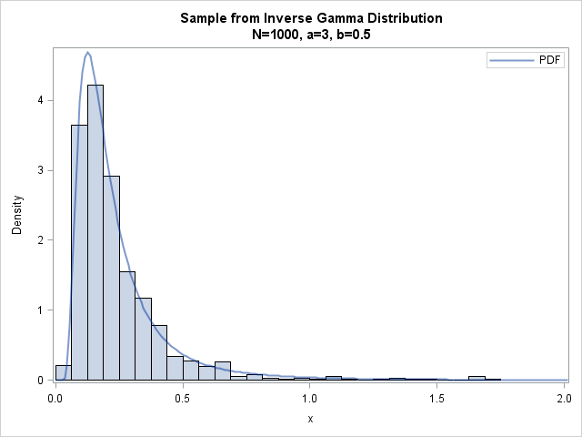
The histogram to the left shows the distribution of 1000 draws from the inverse gamma distribution with parameters a=3 and b=0.5. The PDF of the inverse gamma distribution is overlaid on the histogram. (For details of this technique, see the article "How to overlay a custom density on a histogram in SAS.") The simulated data extend out past x=5, but the histogram and PDF have been truncated at x=2 to better show the density near the mode b/(1+a) = 1/8.

The lesson to learn is that it is often straightforward to use the elementary distributions in SAS to construct more complicated distributions. There are infinitely many distributions, so no software documentation can ever explicitly list them all! However, you can often use elementary arithmetic operations to express a complicated distribution in terms of simpler distributions.