Vector languages such as SAS/IML, MATLAB, and R are powerful because they enable you to use high-level matrix operations (matrix multiplication, dot products, etc) rather than loops that perform scalar operations. In general, vectorized programs are more efficient (and therefore run faster) than programs that contain loops. For an example that demonstrates the relative timing of loops versus vectorized computation, see my previous article on timing performance: looping versus using the LOC function.

For some statistical tasks, it is not obvious how to vectorize the operations. For example, if you want to simulate data from a truncated distribution, the naive approach is to use an acceptance-rejection method, which is not vectorized. I have previously discussed more efficient (vectorized) ways to implement acceptance-rejection algorithms.

Time-series operations can also be hard to vectorize. On discussion forums, people often post programs for time-series analysis that involves scalar computations inside of a loop. Sometimes I am able to contribute a vectorized solution that eliminates the loop by writing the operation in terms of the DIF and LAG functions in the SAS/IML language. This article demonstrates one way to vectorize a time series computation.

Counting the runs in a binary sequence

The following SAS/IML program is similar to one that was posted to a discussion forum. The data are a sequence of binary values, say zeros and ones. A run is a series of consecutive symbols that are the same, such as a sequence of zeros. The goal of the program is to create an indicator variable that identifies to which run each observation belongs. The following 0/1 sequence contains six runs. The sequence and the computed indicator variable are displayed after the program, which uses a loop to compare adjacent elements of the sequence:

proc iml;
b = {1 0 0 0 0 1 1 1 0 1 0};   /* data: a binary sequence with six runs */
 
/* assign a group number for each "run" of a binary observation */
s = j(1, ncol(b), 1);    /* vector of all ones */
do i = 2 to ncol(b);     /* loop over elements; compare adjacent values */
   if b[i]=b[i-1] then   /* if consecutive elements are the same */
      s[i]=s[i-1];       /*    assign the same ID values */
   else                  /* if consecutive elements are different */
      s[i]=s[i-1]+1;     /*    increment the ID value */
end;
print b,s;

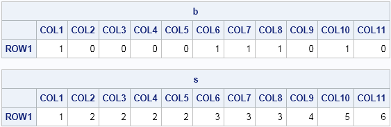
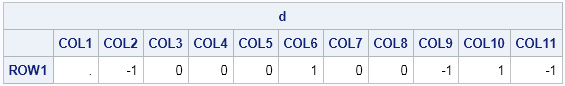
From the table, you can see that the s vector identifies the runs. The last element of s, which is 6, tells how many runs are in the sequence.

Vectorizing the computation

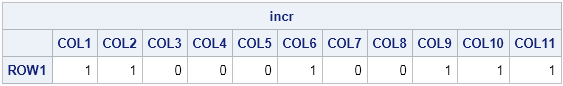
As I mentioned, computations like these can be hard to vectorize. One technique that sometimes works is to use the DIF function to compute the change between adjacent elements. Let's try to vectorize the computation that generates the s vector in the previous section. For a binary sequence of zeros and ones, the difference between adjacent values is +1 or –1 when a new run begins, as shown in the following statements:

d = T(dif(b)); 
print d;

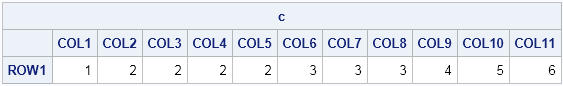
If you don't care about the actual values, but only that the value has changed, then the nonzero values identify the beginning of each run, as follows:

incr = (d^=0);
print incr;

You can use the cumulative sum of these 0.1 values to generate the indicator variable or to count the number of runs:

c = cusum(incr);
print c;

This is the same result as was computed by the loop in the previous section. Therefore, the following one-liner vectorizes the computation that creates an indicator variable for runs in the sequence:

s = cusum(T(dif(b))^=0);    /* vectorized version */

This technique is very useful when dealing with ordered sequences. For example, I previously used this technique to estimate the maximum (or minimum) value of a function, and again to implement the "runs test" to determine whether a sequence is random.

The vectorized computation will be much faster than the loop. For long sequences, the time saved can be significant. So next time that you find yourself writing a loop that computes the difference between evenly spaced elements of a vector, investigate whether you can replace the loop by using the DIF function.