Buffon's needle experiment for estimating π is a classical example of using an experiment (or a simulation) to estimate a probability. This example is presented in many books on statistical simulation and is famous enough that Brian Ripley in his book Stochastic Simulation states that the problem is "well known to every reader" (Ripley 1987, p. 193).

In case the problem is not well-known to you, here's a description of Buffon's needle experiment. (Ripley presents eight modifications of the experiment and analyzes the variance of each estimator, but I will content myself with the simplest description.)

In the experiment, a needle of length L is dropped on a floor that is marked by a series of parallel lines that are d units apart. (Think of a hardwood floor whose boards are width d.) When L ≤ d, elementary trigonometry and calculus shows that the probability that the needle intersects a line is given by P=(L/d)(2/π). If you carry out the experiment (or simulate it), you can estimate the probability by the ratio h/N, where h is the number of times that the needle intersects a line out of N drops. Because you can measure or count all of the constants, you can invert the equation to estimate π.

The case L=d corresponds to the case of a needle that is the same length as the width of the lines. Ripley (1987, p. 194) shows that the variance of the estimator is smallest for this case. You can set d=1 by measuring in units of d. It follows from trigonometry that the needle intersects a line if y ≤ (1/2)sin(θ) where y is the distance from the center of the needle to the nearest line and where θ is the angle the needle makes with the lines. There are dozens of Web sites that derive this result and give diagrams. There are even Web sites where you can simulate dropping a bent needle.

Dropping the needle at random means that y is distributed as U(0, 1/2) and θ is distributed as U(0, π). The following SAS/IML program simulates tossing 1,000 needles of unit length onto a floor with lines spaced one unit apart. The SUM function is used to count the number of times that the needle intersects a line. The variable P contains the proportion of intersections. Because P ≈ 2/π, an estimate of π is 2/P, as shown in the output of the program:

   /* Buffon's Needle */
   proc iml;
   call randseed(123);
   pi = constant("pi");
   N = 1000;
   z = j(N,2);  /* allocate space for (x,y) in unit square */
   call randgen(z,"Uniform"); /* fill with random U(0,1) */
   theta = pi*z[,1]; /* theta ~ U(0, pi) */
   y = z[,2] / 2; /* y ~ U(0, 0.5) */
   P = sum(y < sin(theta)/2) / N; /* proportion of intersections */
   piEst = 2/P;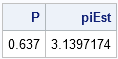
   print P piEst;

In fact, the simulation contains more information than is shown in the table. The simulation provides 1,000 estimates of π! (However, the estimates are not independent of each other.) Notice that you could stop the simulation after 100 trials, or after 200, or after any value. Each potential value of N results in an estimate. The standard error of the estimate is proportional to N^-1/2, so some estimates are better than others. Nevertheless, you can visualize how the Monte Carlo simulation converges by plotting the estimate after N trials against N. You can compute all estimates in a single vectorized operation by using the CUSUM function:

   Trials = T(1:N);
   Hits = (y < sin(theta)/2);
   Pr = cusum(Hits)/Trials; /* Monte Carlo estimates */
   Est = 2/Pr;              /* Monte Carlo estimates of pi */
 
   /* write estimates to a data set */
   create Buffon var {"Theta" "y" "Trials" "Hits" "Est"};
   append;
   close Buffon; 
 
   proc sgplot data=Buffon;
     scatter x=trials y=est;
     refline 3.14159 / axis=y;
   run;

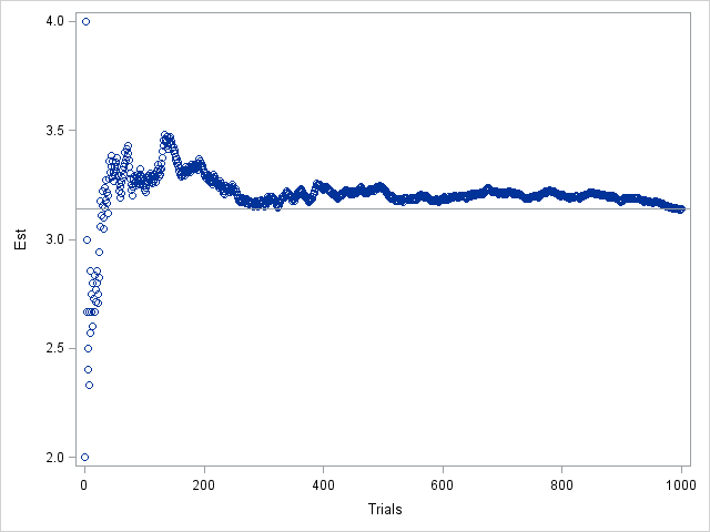
The plot shows that the estimates "bounce around," but approach π for large values of N.

Is this a good way to estimate π? Not particularly. The convergence is rather slow in this "hit-or-miss" method and the variance of this estimator is rather large compared with other integration methods. However, it is a good way to emphasize a few simulation techniques in SAS/IML. Here are three programming tips to take away from reading this article:

• Allocate a vector, then fill it with a random sample. Notice that I do NOT write a loop that iterates N times!
• Use the SUM function to count the number of times that a logical expression is true. Notice that SUM(x)/N is the same as the mean of x, so I could also have used the SAS/IML subscript reduction operator (:) to write P = (y < sin(theta)/2)[:].
• The CUSUM function enables you to form a "running mean." The kth element of Pr is equal to the mean of the first k elements of Hits.