Computer vision is one of the most sought-after artificial intelligence (AI) applications today, finding a wide variety of use cases in image recognition, object detection, biomedical assessment, and more.
SAS supports a diverse set of AI and deep learning capabilities that can be used in many of these applications. One of them is our support for object detection using the popular You Only Look Once (YOLO) algorithm. YOLO algorithms are popular for identifying common objects that can be quickly recognized in a single glance.
This blog post is aimed at creating a good starting point for readers who want to learn the tips and tricks for creating object detection models using AI and deep learning capabilities in SAS® Viya®.
YOLO example background
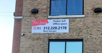
The use case we will be looking at in this post is identifying the location of “FOR RENT/LEASE” signboards in pictures of building and storefronts. Here is a sample training data of the images:

The new SAS Viya platform is significantly more open than traditional SAS platforms in the past. By using Viya’s Cloud Analytics Services (CAS) engine, I am able to code using a variety of interfaces, including R, Python and Java. When using Python, there are two packages that are essential for SAS AI and deep learning capabilities: SWAT and DLPy.
SWAT (SAS Scripting Wrapper for Analytics Transfer) package is the Python client to SAS. It allows users to execute CAS actions and process the results from Python. DLPy (SAS Deep Learning Python API) package is a high-level Python API for the SWAT package. In simpler terms, think about how the Keras API serves as a higher-level abstraction for Tensorflow. DLPy does that for Python. I’ll be using the DLPy package for the example in this post.
9 best practices for YOLO
As we walk through using the YOLO model for object detection, I’ll offer 9 best practices ranging from data management to deployment. Come along on our sign-identifying journey and see what you learn.
1) No double standards!
The YOLO model expects the training images to be of the same dimensions. We have two ways to handle this:
- We can use the CAS action “processImages” using the RESIZE function.
- We can use the CAS action “augmentImages” and explicitly define the “outputWidth” and “outputHeight” parameters.
Since I will be using “augmentImages” in other steps, I chose to resize the images this way.
2) Can I have some more please?
The main prerequisite in any deep learning project is data. A LOT of it. Without a lot of training data you won’t be able to produce a good model. The training set in our use case contained around 120 images. In order to increase the size of my training set, I made use of the “augmentImages” CAS action as previously mentioned. This action performs a variety of image mutations such as random flipping, rotation, image sharpening and coloring, etc while preserving the integrity of the image. Each mutation creates a new image within our training set, increasing the total number of images in the data set from 120 to 315. Here's an example of image augmentation using rotation.
-

- Image before rotation
-

- Augmented image after rotation
3) Truth in labeling
For any good YOLO object detection model, the images need accurate labels. In order to do this, I followed three steps:
- The first step in labeling is drawing bounding boxes around the objects within the image and providing labels for them. To do this, I used an open source package called LabelImg, which is one of the many open source labeling packages available. For this use case, I have labeled the bounding boxes as “sign” to denote the location of the rental/lease signs on buildings. The dimensions of the bounding box(es) for each image will be saved in an XML file and not on the image itself.
- The second step is to choose which format those dimensions will take. SAS supports the following 3 formats for bounding boxes – YOLO, RECT and COCO. For example, if I chose YOLO, the bounding box coordinates would be defined as [xMiddle, yMiddle, width, height]. If I chose COCO, the coordinates would be [xMin, yMin, xMax, yMax].
- The last step is merging each image’s XML file with the image file to create a new image that contains these bounding boxes. In order to do this, place all of the XML files together with the image files into one folder and provide this path location in the “data_path” parameter of create_object_detection_table() method. This method also requires a parameter value for “coord_type”. This would be one of the 3 formats that SAS supports. In my case, I used coord_type = “yolo”.
object_detection_targets = create_object_detection_table( s, image_size=768, data_path='/data /augmented/', coord_type = 'yolo', output = 'trainset') NOTE: Images are processed. NOTE: Object detection table is successfully created |
NOTE: Since the “YOLO” format normalizes bounding box coordinates between 0 and 1, it is not necessary to resize your images even if they are not of the same dimensions. You simply mention the dimensions that you want for your resized image in the “image_size” parameter of the create_object_detection_table() method. However, this is not the case for “RECT” and “COCO.” You need to resize the images before labeling.
4) Get a head start
The process of transfer learning, where you apply a pre-trained model on a new problem, helps alleviate the intense building and training of a deep neural network model from scratch. By using transfer learning, we can now use the weights and biases of a pre-existing model to initialize our model’s own weights and biases. This concept works because learned features are often transferable to different data and doing this saves a lot of time with respect to the actual model building process.
In this example, I am re-using an already existing Tiny Yolo V2 model that was pre-trained on the OpenImagev4 dataset (on images containing not more than 100 objects per image).
5) Anchors away!
Not all objects inside an image will be of the same dimensions. For the YOLO model to adjust to the varying sizes of objects, we need to generate anchor boxes. For every prediction grid, we define a preset number of anchor boxes of predefined shapes and sizes. There will be one anchor box per grid that is responsible for predicting the object whose center lies in that grid. This is determined by finding which anchor box most overlaps with the ground truth bounding box of that object.
Using the get_anchors() method, and specifying the number of anchors per prediction grid(“n_anchors” parameter), I can initialize the height and width of these boxes.
6) You only look once
Before building a YOLO model, I first need to define the architecture. For detailed info on what a Tiny YOLOV2 model architecture should look like, see the documentation on github. Some important things to note:
- The default image size in the documentation is 416x416 pixels. Adjust this parameter to match your image size.
- Predictions are made by dividing an image into square grids each of size 32x32 pixels. Using your image size, determine the size of your prediction grids by dividing your image size by 32.
- The “anchors” parameter should be set to the list of anchor box values that were derived on using the get_anchors() method.
- There are two parameters within the method that often get confused, max_labels_per_image and max_label. The difference between them is:
- max_label_per_image: this denotes the maximum number of bounding box labels that appear in an image in the training set. For example, if you have 3 images with 2 objects each and 1 image with 5 objects, this parameter would be set to 5.
- max_labels: The maximum number of bounding box predictions that you want the model to predict per test image.
7) You Only Look Once (Again)
Now that the model architecture is defined for YOLO, the model training is similar to any other deep neural network training, wherein we specify the appropriate initial weights for the model, the optimizer algorithms, the solver techniques and finally the model fit. There is no hard and fast rule as to what values to provide for these hyper-parameters. We just keep trying different values and see how the training performance changes.
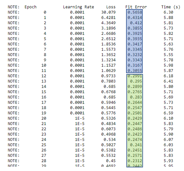
Here is a snapshot of my model training process. To determine if we really have a good model in hand, compare how the loss and fit error change over each epoch. In an ideal model training scenario, one would want both these values to constantly decrease. The Fit error is generally computed in terms of the Intersection over Union (IoU) metric. IoU is a measure of how close the ground truth (i.e., the hand labeled bounding box of an object in a training image) is with the predicted bounding box for that object. Consequently, the higher the IoU value, the more accurate our model is. Fit error is calculated as 1 – IoU. Good object detection models usually see an IoU value over 0.7. So once the Fit error reaches 0.3 or less, you will know that the training is enough.
In the snapshot below, it took 12 epochs for the model to become sufficiently accurate.
8) Score!!!
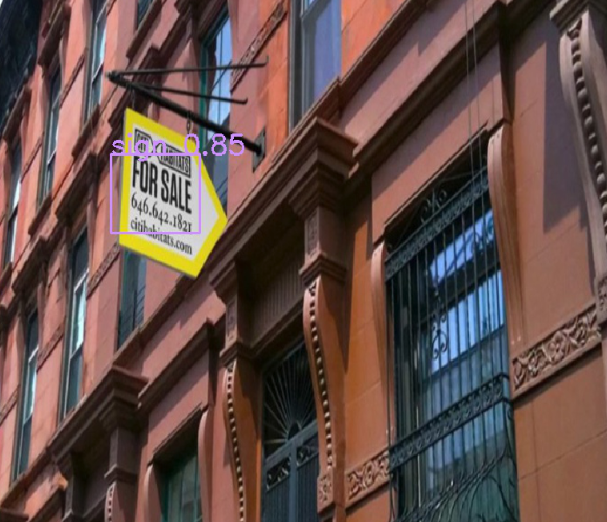
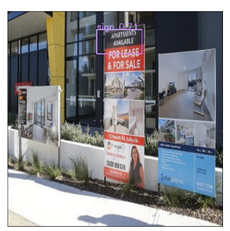
Once the model is trained, it’s time to score the model against validation data. Calling the model.predict() method on the validation dataset saves the model’s predictions along with the validation images in a CAS Table called “model.valid_res_tbl”. To see bounding boxes on validation images, you would use the display_object_detections() method.
display_object_detections(conn=s, coord_type='yolo', max_objects=2, table=yolo_model.valid_res_tbl, n_col=2) |
9) The whole truth and nothing but
The SAS DLPy package also offers the capability to evaluate model performance against scored data. Using evaluate_object_detection() method , and setting your training data set as the “ground truth” parameter, you can evaluate prediction results. This will yield a list of performance metrics for every IoU threshold value such as the precision, recall, and the true positive rate.
Next steps for YOLO
So far, we saw some of the best practices to build and train a YOLO object detection model. Some of the next steps in utilizing this model could be:
- Saving the model weights so it can be used for future transfer learning purposes.
yolo_model = Tiny_YoloV2( s, n_classes=1, model_table = "my_yolo_model", height=768, width=768, predictions_per_grid=5, anchors = yolo_anchors, max_boxes=3, coord_type='yolo', max_label_per_image = 3, class_scale=1.0, coord_scale=1.0, prediction_not_a_object_scale=1, object_scale=5, detection_threshold=0.2, iou_threshold=0.05 ) s.save( table = "my_yolo_model", name = "yolo_model_weights", replace = True ) |
NOTE: Cloud Analytic Services saved the file yolo_model_weights.sashdata in caslib nyc_objdet.
- Saving the model information as a SAS astore file so that it can be easily deployed in RESTful applications or elsewhere.
yolo_model.deploy(path="/tmp",format="astore") |
- Saving the model in ONNX format – The Open Neural Network eXchange is an open format for deep learning models that allows SAS models to be imported into other open source tools such as PyTorch or TensorFlow.Create ONNX of YOLO MODEL
import onnx yolo_model.deploy(path="/tmp",format="onnx") |
NOTE: Model weights will be fetched from server
NOTE: ONNX model file saved successfully
More resources
For more information on using SAS Deep Learning capabilities for building YOLO object detection models, visit our SAS-DLpy Github or watch the video below.


3 Comments
Great post, thanks!
Good job. Neela
Thanks for the great article! The data science community will definitely find it helpful!
Best,
365 Data Science
365 Data Science is an online educational career website
https://365datascience.com