
The computer vision team was recently presented with the following challenge concerning image matching performance. An insurance company has the capability to submit claims and supporting materials digitally via an online interface. They need, however, to be able to detect when images already used in previous claims have been resubmitted for use in new claims. Basically, someone submits the same image of vehicle damage to two separate accident claims to receive double the insurance money. The detection of exact duplicates is a task that can already be handled easily. However, submitting slightly altered versions of the same image is the issue. The insurance company needs a more robust way to scan images that will detect the slightest of modifications. Examples would include scaling, rotation, translation, blurring, and cropping.
This type of image processing is much more computationally intensive. So much so it can be very difficult, or even impossible, for the insurance provider to perform this type of scan at a pace that keeps up with all the new images being submitted. Motivated by the need to scan incoming images quickly and effectively, we will use SAS Viya to solve the problem of intelligently searching for new images among a large database of old images.
Introducing two SAS Viya image processing tools
There are two image-processing tools available in SAS Viya that we will leverage to address the problem of efficiently matching similar images.
The matchImages Action
The matchImages action provides robust methods for searching for an image within a collection of images. By robust, we mean that the action can match similar images, even if image variations of the sort discussed earlier are present. The matchImages action provides this by measuring the similarity between images using scale- and rotation-invariant keypoints. This means that images need not be exact duplicates in order to be matched. Instead, pairs of similar images might be matched even when one is a scaled, rotated, or even a cropped version of the other.
As mentioned previously, these types of modifications would by no means be unexpected in the insurance fraud scenario. So the matchImages action lends itself well to the problem. However, this kind of robustness comes at a cost – finding and describing keypoints in images is a computationally intensive exercise. An insurance company’s claims database already contains millions of images while hundreds of new images are submitted daily. So the approach of using matchImages alone to repeatedly compare newly-submitted images against their entire database of images is infeasible. To keep pace with new image submissions, something else is needed to make the analysis more efficient.
The quantifyImages Action
Among the new functionality that appeared with the release of SAS Viya 4 is the quantifyImages action. In a nutshell, this action provides numerical values derived from the characteristics of images. The action currently supports five quantity types, but plans are already in place to add more. Of the quantity types presently supported, four provide metrics related to the pixel value distributions of each image channel. This is namely their minima and maxima as well as their means and standard deviations. In comparison to finding image keypoints and computing their descriptors, these metrics are extremely easy to compute. What if we used these metrics to intelligently reduce the search space for the matchImages action call? In essence, the idea is to exploit inexpensive computations on the front end to reduce the number of expensive computations required on the back end.
Demonstration scenario for image matching
For our demonstration using the quantifyImages action capabilities, we will be using 200,000 images from the Google OpenImagesV4 dataset. These are images with no uniformity – no specific type of content, some multichannel (color) and some single-channel (grayscale) images, and all of varied sizes. We randomly select all but 100 images to form the image database. That means there's a total of 199,900 images in the CAS table database_images.
Next, we take the 100 images that were excluded in the previous step. We add 100 random images that were included in the image database to create a collection of 200 images in the CAS table given_images. This is named so because these would represent the new images given by a customer. Tying it back to the insurance scenario, these would be the images uploaded by an insurance customer in support of a claim. The code in the subsequent sections will search the database for images that match these 200 images quickly and accurately.
Brute-force approach
To establish a baseline, we will first demonstrate the brute-force approach. This just means to call matchImages for every given image and search for it among the entire database of existing images. This would likely represent the approach taken before the introduction of the quantifyImages action.
# Store the output of matchImages in the following table. match_images_output = cas.CASTable(name='match_images_output') for current_row in range(0, given_images_paths.shape[0]): # For the current row, extract the filename from the long absolute path. current_path = os.path.basename(given_images_paths[current_row]) # Call matchImages, specifying the current path as the template image. result = cas.image.matchImages( image=current_path, table=database_images, casout=cas.CASTable(match_images_output, replace=True), threshold=0.6, highlight=False ) |
You might be wondering about the threshold parameter in the matchImages action call. This parameter allows us to look not just for the exact duplicates but allows two images to be deemed duplicates as long as they fall within the similarity threshold. This is what enables matchImages to detect approximate matches. Mapping the threshold value to a qualitative explanation of similarity isn’t possible. In practice, the threshold would be selected after some trial and error. All of the code today uses a threshold of 0.6, which comes from an actual threshold value used by one of our customers.
Now, let’s evaluate the performance of this baseline. On the CAS grid used throughout this study, the brute-force approach required an average search time of 38.3 seconds per image. This resulted in a 20.2% mismatch rate. That is, slightly over 20% of the given images were either deemed duplicates when they were actually unique. Or they were deemed unique when they should have been flagged as duplicates. Unfortunately, this baseline performance is not sufficient. Not only are one out of five images misclassified, but it takes nearly 40 seconds to scan an image against a toy image database that’s much smaller than what would be encountered in practice. Something more is needed to create a viable solution.
Precomputing metrics for the image database
In order to develop more viable solutions, we will intelligently reduce the search space considered by the matchImages action. To decide which images to include and exclude, we need data on which to base our decisions. The quantifyImages action is well-suited to providing these data. As discussed earlier, the quantifyImages action can compute metrics based on image characteristics. Here, we look at computing and storing these image metrics for the image database. Later, we exploit these metrics to reduce the search space and yield viable solutions. In the following code snippet, we compute four different types of quantities for each of the images in the image database using a single call to quantifyImages.
# Store the output of quantifyImages for database_images in the following table. database_images_quantified = cas.CASTable(name='database_images_quantified') # Quantify database_images. cas.image.quantifyImages( images=dict(table=database_images), quantities=[ dict(quantity=dict(quantitytype='mean')), dict(quantity=dict(quantitytype='std')), dict(quantity=dict(quantitytype='minimum')), dict(quantity=dict(quantitytype='maximum')) ], copyvars=['_image_'], casout=cas.CASTable(database_images_quantified, replace=True) ) |
The result is a CAS table, database_images_quantified, with thirteen rows, one for the image and one for each metric and channel (4 metrics across 3 channels yields 12 total values). In the following sections, we will use these twelve new columns to methodically exclude images from the matchImages search space.
Reducing the search space using minimum and maximum pixel values
Now we will use knowledge of pixel value extremes as a simple initial way to reduce the number of images searched through by matchImages. Specifically, we will ask quantifyImages to find the minimum and maximum pixel values for each given image. Then we use a where clause to limit the search space of the matchImages call to only those images in the database whose corresponding metrics are within 10% of those values. This approach is illustrated in the code snippet below.
# Store the output of quantifyImages in the following table. quantify_images_output = cas.CASTable(name='quantify_images_output') # Store the output of matchImages in the following table. match_images_output = cas.CASTable(name='match_images_output') # Define the names of the columns containing the quantities of interest. quantity_columns = ['_channel1minimum_', '_channel2minimum_', '_channel3minimum_', '_channel1maximum_', '_channel2maximum_', '_channel3maximum_'] for current_row in range(0, given_images_paths.shape[0]): # For the current row, extract the filename from the long absolute path. current_path = os.path.basename(given_images_paths[current_row]) # Define a new given_image table containing just the current image within given_images. given_image = cas.CASTable( given_images, where=given_images.where + " and _path_ = \"" + given_images_paths[current_row] + "\"" given_images_paths[current_row] + "\"" ) # Call quantifyImages on the current given_image. cas.image.quantifyImages( images=dict(table=given_image), quantities=[ dict(quantity=dict(quantitytype='minimum')), dict(quantity=dict(quantitytype='maximum')) ], casout=cas.CASTable(quantify_images_output, replace=True) ) # Retrieve the quantified values. quantify_images_values = cas.table.fetch( table=quantify_images_output )['Fetch'] # Reset the refined where clause. refined_where_clause = "" # Loop through the quantities of interest to create the refined where clause. for quantity_column in quantity_columns: # Get the given image's value for the current quantity. value = quantify_images_values[quantity_column][0] # If it's not-a-number, skip it. if(numpy.isnan(value)): continue # Compute the tolerance for the current quantity. tolerance_percentage = 10 tolerance = tolerance_percentage/100 * abs(value) # Refine the where clause. refined_where_clause = refined_where_clause + " and " + quantity_column + " >= " + str(value - tolerance) + " and " + quantity_column + " <= " + str(value + tolerance) # Fence post problem - remove the beginning of the where clause. refined_where_clause = refined_where_clause[5:] # Define the refined database images table. refined_database_images = cas.CASTable(database_images_quantified, where=refined_where_clause) # Call matchImages, specifying the current path as the template image and searching through the refined_database_images table. result = cas.image.matchImages( image=current_path, table=refined_database_images, casout=cas.CASTable(match_images_output, replace=True), threshold=0.6, highlight=False ) |
Using these simple metrics, the average search time per query image is reduced from 38.3 seconds to 21.5 seconds. This is a reduction of nearly 44%. Note we previously compared to the full database but using quantifyImages allowed us to narrow down the search space. Here we only compare the query image against a subset of the full database.
Without the addition of much computational burden, we have intelligently reduced the search space. This means that there are a lot of highly complex keypoint descriptor vectors that are now not being computed. That’s where the gains are found in search time and start to really improve the feasibility of operating a robust image matching system. The benefits don’t stop there, however. Not only are the search times reduced, but the mismatch rate has also decreased slightly to 15.8%. This represents a 21.5% reduction in mismatches compared to the baseline brute-force approach.
Reducing the search space using all available metrics
There are two other quantity types available to us, namely the pixel value means and standard deviations. So let’s focus on them and take a look at how using their values can impact image matching performance. The general approach is as before. Only those images in the database whose precomputed metrics lie within 10% of the given images’ corresponding values are considered in the matchImages comparisons.
# Store the output of quantifyImages in the following table. quantify_images_output = cas.CASTable(name='quantify_images_output') # Store the output of matchImages in the following table. match_images_output = cas.CASTable(name='match_images_output') # Define the names of the columns containing the quantities of interest. quantity_columns = ['_channel1mean_', '_channel2mean_', '_channel3mean_', '_channel1std_', '_channel2std_', '_channel3std_'] for current_row in range(0, given_images_paths.shape[0]): # For the current row, extract the filename from the long absolute path. current_path = os.path.basename(given_images_paths[current_row]) # Define a new given_image table containing just the current image within given_images. given_image = cas.CASTable( given_images, where=given_images.where + " and _path_ = \"" + given_images_paths[current_row] + "\"" ) # Call quantifyImages on the current given_image. cas.image.quantifyImages( images=dict(table=given_image), quantities=[ dict(quantity=dict(quantitytype='mean')), dict(quantity=dict(quantitytype='std')) ], casout=cas.CASTable(quantify_images_output, replace=True) ) # Retrieve the quantified values. quantify_images_values = cas.table.fetch( table=quantify_images_output )['Fetch'] # Reset the refined where clause. refined_where_clause = "" # Loop through the quantities of interest to create the refined where clause. for quantity_column in quantity_columns: # Get the given image's value for the current quantity. value = quantify_images_values[quantity_column][0] # If it's not-a-number, skip it. if(numpy.isnan(value)): continue # Compute the tolerance for the current quantity. tolerance_percentage = 10 tolerance = tolerance_percentage/100 * abs(value) # Refine the where clause. refined_where_clause = refined_where_clause + " and " + quantity_column + " >= " + str(value - tolerance) + " and " + quantity_column + " <= " + str(value + tolerance) # Fence post problem - remove the beginning of the where clause. refined_where_clause = refined_where_clause[5:] # Define the refined database images table. refined_database_images = cas.CASTable(database_images_quantified, where=refined_where_clause) # Call matchImages, specifying the current path as the template image and searching through the refined_database_images table. result = cas.image.matchImages( image=current_path, table=refined_database_images, casout=cas.CASTable(match_images_output, replace=True), threshold=0.6, highlight=False ) |
This approach yields very significant improvements in performance. The average search time per image is down to only 2.0 seconds, which is a nearly 95% reduction compared to the baseline. Furthermore, the mismatch rate is down to 5.3%, a 73.6% reduction compared to using the entire unfiltered database of images. Being able to accurately scan about 20 times as many images as before can really go a long way in the battle to process images at the pace at which they arrive.
Reducing the search space using pixel distribution metrics
In this section, we look at the approach that’s likely already been on most readers’ minds. That is, using all four aforementioned metrics and observing their impact on search time and accuracy. Given how helpful the means and standard deviations proved themselves to be in the previous section, running the following code will demonstrate whether additional gains are possible when they are combined with pixel value extremes in order to narrow down the search space.
# Store the output of quantifyImages in the following table. quantify_images_output = cas.CASTable(name='quantify_images_output') # Store the output of matchImages in the following table. match_images_output = cas.CASTable(name='match_images_output') # Define the names of the columns containing the quantities of interest. quantity_columns = ['_channel1mean_', '_channel2mean_', '_channel3mean_', '_channel1std_', '_channel2std_', '_channel3std_', '_channel1minimum_', '_channel2minimum_', '_channel3minimum_', '_channel1maximum_', '_channel2maximum_', '_channel3maximum_'] for current_row in range(0, given_images_paths.shape[0]): # For the current row, extract the filename from the long absolute path. current_path = os.path.basename(given_images_paths[current_row]) # Define a new given_image table containing just the current image within given_images. given_image = cas.CASTable( given_images, where=given_images.where + " and _path_ = \"" + given_images_paths[current_row] + "\"" ) # Call quantifyImages on the current given_image. cas.image.quantifyImages( images=dict(table=given_image), quantities=[ dict(quantity=dict(quantitytype='mean')), dict(quantity=dict(quantitytype='std')), dict(quantity=dict(quantitytype='minimum')), dict(quantity=dict(quantitytype='maximum')) ], casout=cas.CASTable(quantify_images_output, replace=True) ) # Retrieve the quantified values. quantify_images_values = cas.table.fetch( table=quantify_images_output )['Fetch'] # Reset the refined where clause. refined_where_clause = "" # Loop through the quantities of interest to create the refined where clause. for quantity_column in quantity_columns: # Get the given image's value for the current quantity. value = quantify_images_values[quantity_column][0] # If it's not-a-number, skip it. if(numpy.isnan(value)): continue # Compute the tolerance for the current quantity. tolerance_percentage = 10 tolerance = tolerance_percentage/100 * abs(value) # Refine the where clause. refined_where_clause = refined_where_clause + " and " + quantity_column + " >= " + str(value - tolerance) + " and " + quantity_column + " <= " + str(value + tolerance) # Fence post problem - remove the beginning of the where clause. refined_where_clause = refined_where_clause[5:] # Define the refined database images table. refined_database_images = cas.CASTable(database_images_quantified, where=refined_where_clause) # Call matchImages, specifying the current path as the template image and searching through the refined_database_images table. result = cas.image.matchImages( image=current_path, table=refined_database_images, casout=cas.CASTable(match_images_output, replace=True), threshold=0.6, highlight=False ) |
As it turns out, further gains are possible. Using all four quantity types, the average search time is brought to 1.5 seconds and the mismatch rate is down to 3.7%. As a whole, these numbers show that the full-filtering approach yields a 96% reduction in search time. As well as an 81.8% reduction in mismatches when compared to the baseline approach. These are very significant gains at very insignificant computational costs.
Image matching performance conclusion
In this post, we've demonstrated how the quantifyImages and matchImages actions can be combined and efficiently applied to solve a real-world image matching problem. This results in not just significant performance gains, but even taking something that was originally infeasible and turning it into something feasible. In the following graph, we summarize the gains observed throughout this discussion.
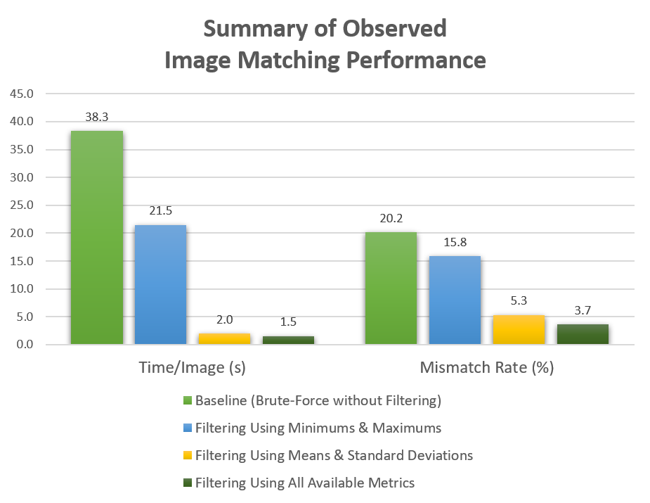
As seen above, different and more quantities are used to filter the search space considered by the computationally complex matching algorithm. This shows the remarkable performance improvements in our image matching demonstration scenario. In reference to the insurance fraud scenario, the image database in this demonstration is likely much smaller than a real-world scenario. We anticipate that an even greater positive impact would be observed when these methods are applied to real customer databases. In conclusion, the analysis here showcases that applying simple metrics can make all the difference. It creates an approach that is very viable and extremely effective instead of one that is prohibitive and infeasible.
LEARN MORE | SAS Viya


1 Comment
Pingback: A million images a minute: a behind-the-scenes look at the loadImages action in SAS Viya - The SAS Data Science Blog