A note from Udo Sglavo: When people ask me what makes SAS unique in the area of analytics, I will mention the breadth of our analytic portfolio at some stage. In this blog series, we looked at several essential components of our analytical ecosystem already. It is about time to draw our attention to the fascinating field of econometrics. Xilong Chen, Senior Manager in Scientific Computing R&D, will share his excitement and passion for a rapidly evolving area of modern data science. Which ingredients do we need to consider to create modern econometrics software? Let’s hear from Xilong.
Econometrics: What does it mean?
There are many definitions of econometrics. Going to its origins, the word econometrics originated from two greek words: oikonomia, meaning the study of household activity and management, and metriks, which stands for measurement. Modernizing the definition, we arrive at econo-metrics, the measurement and testing of economic theory by using mathematics, statistics, and computer science knowledge. Discussing econometrics, I jokingly say that it can be defined as: Economics = Mathematically Checked and Conveyed (E=MC2). Development of economic theory and its applications has spanned centuries. Let's take a look at the history of this specialty.
How did modern econometrics evolve?
In this post, I will discuss some of the applications of modern econometrics. The road to forming and establishing modern econometrics was a long and complicated one. Many things changed over the hundreds of years due to advancements in statistical, mathematical, and computer science theory However, the dominant driver of the change was technology related. Regression remained the workhorse of econometrics, but it became much more complex due to attempts for large scale modeling and availability of big data. Technology, including grid and cloud computing, enabled us to crunch a lot of data but it is often not enough just to rely on technology. When there is a lot of data, TECHNOLOGY itself is not enough---you need “tricks”, which I will talk about next.
Large data and large models? SAS Econometrics has tricks.
We can use spatial regression as an example of large data and large models Spatial regression is based on the first law of geography (Tobler 1970): “Everything is related to everything else, but near things are more related than distant things.”
Using regression, you can construct a model projecting the target variable of interest at one location on regressors at the same location and, at the same time, regressors at neighboring locations. It is still a regression but enhanced by neighboring relationships that play an essential role. These neighboring relationships are recorded in a matrix that can be quite large. In spatial econometrics we call it the matrix of spatial neighbors (weights) that directly depends on the number of locations that enter the analysis.
For example, performing analysis involving US census data at the tract level contains 64,999 locations (tracts). Not a large number on its own but the problem we are solving becomes large if each of these locations can potentially interact with other locations. If we try to record these relationships fully, it means that the dimension of the spatial weight matrix is 64,999 by 64,999. If you directly read this matrix into memory, it needs about 30GB. Even if you have enough memory to accommodate a matrix of that size on your computer, there is no doubt that the computation speed will be greatly impacted when you perform computations with such a large matrix. You might not have enough hours in the day to solve your model!
Considering the difficulties that might arise when dealing with large matrices, it might be time to think about some tricks and answer questions that can help you to make the problem to become much computationally simpler.
The first thing to consider would be the sparsity of the matrix. We can likely take advantage of the fact that the weight matrix is sparse. Really it means that there are not that many possible neighbors for each of its elements (not everyone can be a neighbor with everyone else) and you only store the relevant ones. The sparsity trick might get you over the problem of storing the matrix. With this sparse representation trick, you are able to store it in memory.
But it is likely that you still need to work with this matrix of NxN size in your calculations. For example, you might need to take an inverse of this matrix, possibly doing this more than once. Assuming it is computationally feasible, inversing the matrix with billions of elements would take many CPU hours. It would be time to use another trick and think about altering your calculation through an approximation that avoids the inversion of the matrix. Both tricks (and many more) have been applied in the CSPATIALREG procedure in SAS Econometrics. You can get your estimation result quickly and accurately for very large problems.
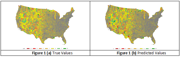
Figure 1 (a) and (b) below are the images of true values vs. predicted values for the analysis of census tract data with very large matrix of spatial neighbors. PROC CSPATIALREG uses the Taylor approximation and finishes the estimation in about one minute, instead of days or months that it would take if the full estimation method was used. The predicted values are very close to the true values.
Going big with time-series modeling
One big branch of econometrics is time series analysis. Some scholars even think the econometrics field started with time series analysis. I like to call the goals of time series analysis “UFO”:
- Understanding the past.
- Forecasting the future.
- Optimizing the present.
There are many applications of time series analysis in different fields. There is one example in the stock market that is fairly difficult to model. You might be familiar with the concept of a bull market and a bear market. If you knew when it was to be a bull or bear market, trading might be much easier. Unfortunately, the market states cannot be directly observed. What you can observe is the stock prices. How do you decode the hidden states from what you can observe? Hidden Markov Models (HMMs) to the rescue!
Why do I call HMM a big model? Because HMM explores the probability space in an exponential way. For example, from 1926 to 1999, there were about 4,000 business weeks. Assume that HMM uses two hidden states to model weekly data, then, there are 24,000 possible paths of hidden scenarios due to the combination of these two hidden states along 4,000 weeks! In such an insanely large modeling space, HMM can find out which path is the most likely one by applying the trick (the Viterbi algorithm) to decode the hidden states so you can “observe” them.
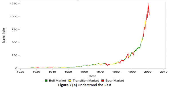
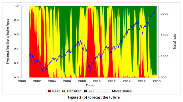
Figure 2 (a) describes three hidden market states: bull, bear, and in-between. The estimation and model selection are another huge task. In this example, it costs about 10,000 CPU hours to find the best HMM. Once the best model is found, you can apply it to the new data (from 2000 to 2017 in this example) to forecast next week’s market state for each time window in the new data. Then you can define your trading strategies according to such forecasts---optimizing the present. The forecasts and wealth curves of different trading strategies are shown in
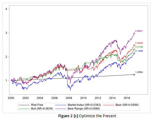
Figure 2(b) and 2(c), respectively. In this example, by using HMMs to design your trading strategies, you can beat the market by 70% better in return, or 70% better in Sharpe Ratio! For more information, see Example 14.1 Discovering the Hidden Market States by Using the Regime-Switching Autoregression Model in the chapter The HMM Procedure.
Big simulation anyone?
This example covers a modern and important simulation method in the area of Bayesian analysis and MCMC (Markov Chain Monte Carlo). I’m going to talk briefly about Bayesian Analysis of Time Series (BATS), and eventually about something even more complex than MCMC---the SMC, the Sequential Monte Carlo method, which is also known as the particle filter. The concept is related to Kalman filter, a well-known technique for the (linear Gaussian) state space models (SSMs). The particle filter extends the filtering framework to nonlinear non-Gaussian state space models.
SSM play a critical role in time series analysis, because many time series models can be written in the state space form, such as ARIMA, UCM, VARMA, stochastic volatility models, and so on. In this example, I will use the Stochastic Susceptible-Infected-Recovered (SSIR) model for the COVID-19 pandemic to demonstrate modern SMC analysis.
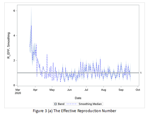
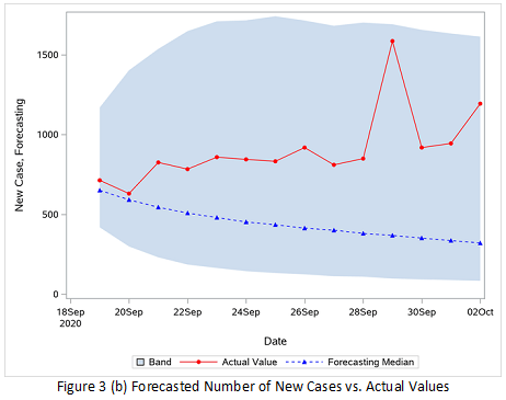
In the epidemic theory, the effective reproduction number, R, is an extremely important parameter. R is the average number of secondary cases per primary case. The R is time-varying due to the epidemic spread stage, intervention, and other factors. Once R < 1, it implies that the epidemic might be in decline and under control. How to trace R along the time is not an easy task, and the SSIR model is one way to do so. However, due to the nonlinearity in the modeling, there is no closed-form solution, so we need to use some approximation methods and SMC certainly comes to mind. Based on the real COVID-19 data for Pennsylvania and through millions of or even billions of simulations, the R can be traced, as shown in Figure 3 (a), and the future number of new cases can be forecasted and compared with the actual values, as shown in Figure 3 (b). The effective reproduction number is successfully traced even with the confidence intervals. Forecasts are very accurate since the true testing data are within the confidence intervals of forecasts.
For more information, see Example 18.3 Estimating the Effective Reproduction Number of COVID-19 Cases in Pennsylvania in the chapter The SMC Procedure.
No small problems
I often say that there are no “small” problems in econometrics. Some problems might be larger than others. However, if you have the right toolbox you can solve them all. SAS Econometrics, including SAS/ETS, offers a lot of value. I encourage you to explore the SAS Econometrics offering for your daily modeling needs.
Procedures Doc | SAS Econometrics
For more information about spatial regression analysis, watch the video Spatial Econometric Modeling for Big Data Using SAS Econometrics or the tutorial SAS Introduction to Spatial Econometric Modeling.
This is the eighth post in our series about statistics and analytics bringing peace of mind during the pandemic.