Whether you’re applying for your first credit card or shopping for a second home – or anywhere in between – you’ll probably encounter an application process. As part of that process, banks and other lenders use a scorecard to determine your likelihood to pay off that loan.
Naturally, this means credit scoring is an important data science topic for banks and any business that works with the banking industry.
Since I have previous experience with customer analytics, but not specifically with financial risk, I’ve been learning how to develop a credit scorecard, and I wanted to share what I’ve learned including my thoughts and code implementation.
Scorecards and the value of credit scoring
There are two basic types of scorecards: behavioral scorecards and application scorecards.
- Behavioral scorecards deal more with predicting or scoring current customers and their likelihood to default.
- Application scorecards are used when new customers apply for loans to predict their likelihood to be profitable customers, and to associate a score to them.
For banks, credit scoring helps manage risk. As consumers we’re bombarded with offers. It’s up to the business to assess the credit worthiness and credit scores of consumers to identify optimal product solutions based on risk, turnaround times, incorrect credit denials and more.
If credit is offered when it shouldn’t be, then a future loss is likely. If turnaround times to approve or deny credit have long lag times or a bank inaccurately denies a good customer credit, they could lose those customers to competitors. In those situations, it might be a long time before you get them back.
Using credit scoring can optimize risk and maximize profitability for businesses.
Credit scoring data
The training data for the credit scoring example in this post is real customer bank data that has been massaged and anonymized for obvious reasons. The features - what are called characteristics in credit scoring - include the number of children, number in household, age, time at address, time at current job, has a telephone, income, etc. Our target variable will be a binary variable with the values ”bad” or ”good” with respect to the customer defaulting given some historical period.
The credit scoring code
For this analysis I’m using the SAS Open Source library called SWAT (Scripting Wrapper for Analytics Transfer) to code in Python and execute SAS CAS Action Sets. SWAT acts as a bridge between the python language to CAS Action Sets. CAS Action Sets are synonymous to libraries in Python or packages in R. The one main difference and benefit is that the algorithms within these action sets have been highly parallelized to run on a CAS (Cloud Analytic Services) server. The CAS server is a distributed in-memory engine where I can do all my heavy lifting or computations. The code and Jupyter Notebook are available on GitHub.
The credit scoring method
Weight of evidence
I first transform my data using the weight of evidence (WOE) method. This method attempts to find a monotonic relationship between the input features and your target variable by splitting each feature into bins and assigning a weight to each bin. Suppose a WOE transformation on income level included income level $100k - $150k, then all observations within that bin would receive the same WOE value which can be computed using the formula below.
\(woe \:value = ln \left( \frac{\% Good}{\% Bad} \right) * 100\)
Weight of Evidence Calculation
Consider a bin for income level between $100k – $150k. Of all the "good" observations in our data, 30 percent come from this income level bin while only 10 percent of the "bad" observations come from this bin. Using these proportions, you could state that we have 3:1 odds that a person between the income of $100k and $150k is a good credit candidate versus bad. We then take the natural log and multiple by 100 for easier numeric representation and we have our WOE value for income level for all observations that fall within our income level bin.
\(ln \left( \frac{0.30}{0.10} \right) * 100 = 109.86\)
Weight of Evidence Example
Data pipeline
Let’s apply this transformation to our entire data set. Using the data preprocess action set in SAS makes it very easy to build data pipelines (Figure 1). Data pipelines help the flow of automation of common manual data science steps. This action set can build out large data pipelines for a variety of transformations across any continuous or nominal features.
There are only a few steps to building a single pipeline:
- Assign variables to roles.
- Build variable transformations.
- Append transformations to later apply to data.
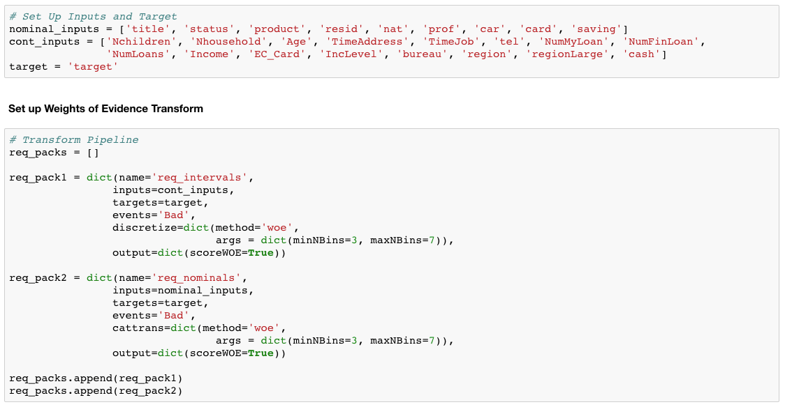
First, we assign the features to their roles, with respect to the transformation and modeling, separating nominal and continuous variables as well as the target (Figure 1)

Next, we create the first transformation called req_pack1, which is just short for request package and is the parameter found in the datapreprocess.transform action. I give that transformation a name, pass the list of features and the target, and specify the event of interest, which is ”bad” in this case.
I call discretize in Python to bin the continuous values and specify the WOE transformation. Within that transformation is a regularization parameter where you can specify a range of bins using the min and max NBins parameter. This enables a search across those bins to find the optimal bin number using information value (IV). IV is a common statistic used in classification models to gauge the predictive power of your feature set.
The second transformation, which I label as req_pack2, is nearly identical except I’m transforming the nominal inputs and therefore need to use cattrans instead of discretize. The cattrans parameter stands for categorical transformation.
We then append those lists together to later pass the transformation outline to our transform action.
Data Transformation
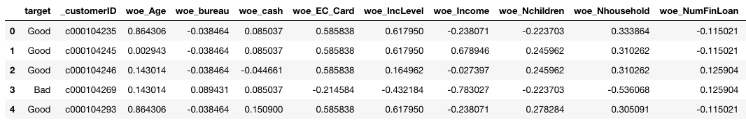
Now that we have our data pipeline in place, let’s transform the data (Figure 3). I first reference our data using the table parameter. Then I provide the req_packs list that I created in figure 2 with all the transformations. I specify the output table (casout) to be called woe_transform. Next, I use copyVars to copy the target and _customerID feature over to our new transformed table from the original table. Then I give a global prefix of “woe” to all our newly transformed features. The code parameter saves the transformation as a code table. This will be used later for scoring new data. This benefits teams that want to do model collaboration or build out deeper end-to-end pipelines for reoccurring jobs.
Finally, we’ll look at a preview of our new WOE table (Figure 3). Notice the identical values for some of our customers. Remember this happens because those observations, for a given variable, fall into the same bin and therefore receive the same weight.
![]()
Visualizing transformation results
The transform action creates several output tables on the CAS server like the one from Figure 3. One of those tables is called VarTransInfo, which contains the IV statistic for our features. Its good practice to look at IV for our features to understand their predictive power and to determine if it’s necessary to include those features in our model. Below is the calculation for IV. Figure 4 is a plot of those IV values for each of our features. Strong features typically have an IV > 0.3, weak features < 0.02, and anything > 0.5 may be suspicious and need a closer look. Figure 4 shows that our features almost split in half between strong and then somewhere in the middle. Also, the age variable looks suspiciously strong. For now, we’ll keep all the features.
\(Information \: Value = \sum (\% \: of \: nonevents - \% \: of \: events) * WOE\)

We can also plot the WOE values of our features by their assigned bins. Aside from viewing these WOE values across bins, a data scientist may want to go back and manually configure the number of bins (combining or splitting up) per a specific variable that makes more logical sense. It’s important to know that WOE attempts to create separation within individual features as it relates to a target variable so there should be differences across bins. Figure 5 shows WOE values that you would expect to see across bins indicating separation within those features.
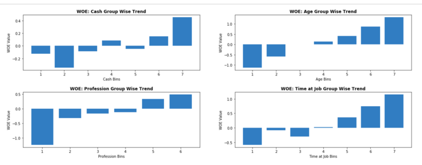
This is really where a data scientist needs to understand the business in order to ensure the weighting trend across bins is logical. For example, it makes business sense to a bank that the more cash a customer has available that it should see a higher weighting across bins. The same type of logic applies to time at a job, age, or profession group. We would expect all of those weightings to be higher with respect to the bins.
Logistic regression for scorecards
The next step we have is to fit a logistic regression model using our newly transformed WOE dataset. I will show the very easy code to train the model and explain the parameters.
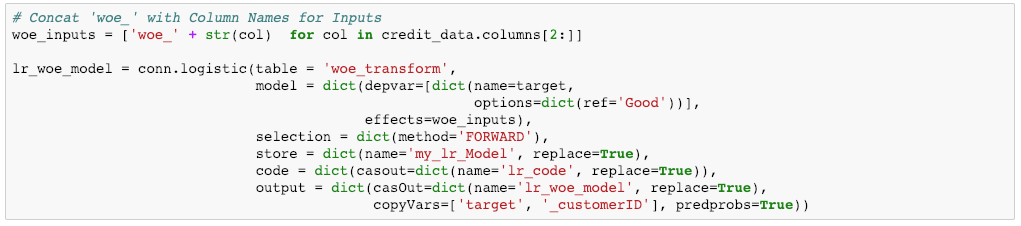
Figure 6 below shows the training code. Here are the steps involved for training the model:
- Assign model inputs and concatenate “woe_” to all original column names so it references the woe_transform dataset correctly.
- Reference the woe_transform dataset using the table parameter.
- Specify the target as well as the reference (reference ‘good’ or ‘bad’ in terms of the model).
- Then, specify forward selection method for variable selection. Forward selection starts with an empty model and adds a single variable at each iteration based on a specific criterion (AIC, AICC, SBC, etc.).
- Use the code parameter to save our logistic regression code
- Create a name for the new output table using casout and then copy over the target and _customerID variables again.
Creating the scorecard
The final step is to scale the model into a scorecard. We’ll be using a common scaling method. We’ll need both our logistic regression coefficients that we got from fitting our model as well as our WOE dataset with the transformed WOE values. We’ll score our training table to derive the logit or log odds values. Since our score from a logistic regression is in log odds form we need to convert that to a point system for our scorecard. We do that conversion by applying some scaling methods.
The first value is the target score. This can be considered a baseline score. For this scorecard we scaled the points to 600. The target score of 600 corresponds to a good/bad target odds of 30 to 1 (target_odds = 30). Scaling does not affect the predictive strength of the scorecard, so if you select 800 as your score for scaling it won’t be an issue.
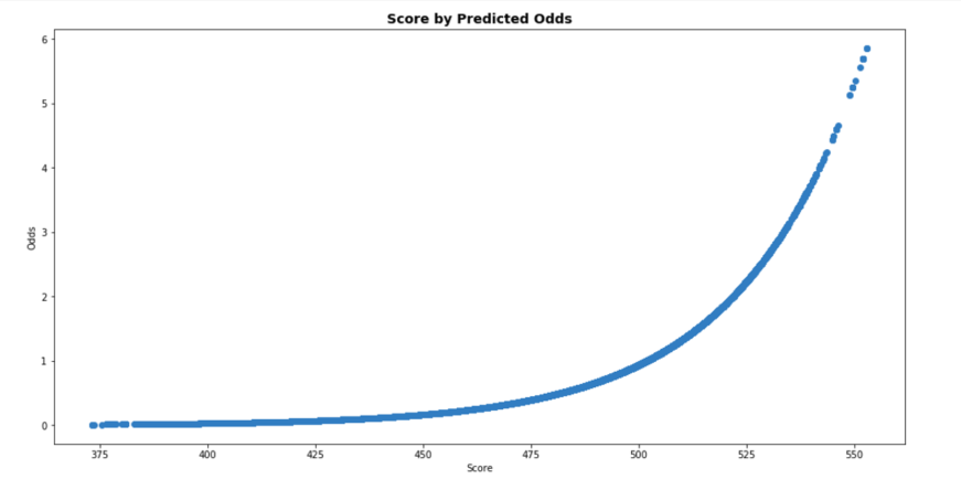
The next variable is called pts_double_odds which means points to double the odds. This means that a score with an increase of 20 points doubles our odds that the applicant is good in terms of default. For example, if you have a score of 600 you have 30 to 1 odds of being a good credit candidate. But a score of 620 raises you to 60:1 odds of being considered good. Figure 8 below shows a visualization of the exponential relationship between predicted odds and score. Below in Figure 7 you can see the simple calculations and how they’re used to derive our scorecard score variable.

Visualizations
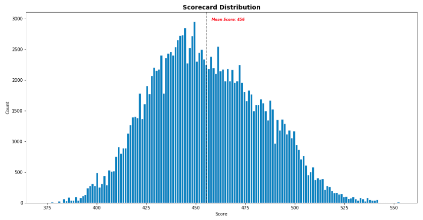
We can look at a distribution of the scorecard score variable here in Figure 9 with the mean score being 456.
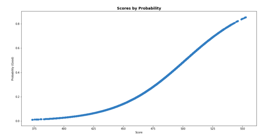
And then we can also see how those scores correlate to our probability of being good or bad credit customers for our business, in Figure 10. You can see the nice sigmoidal shape of the plot.
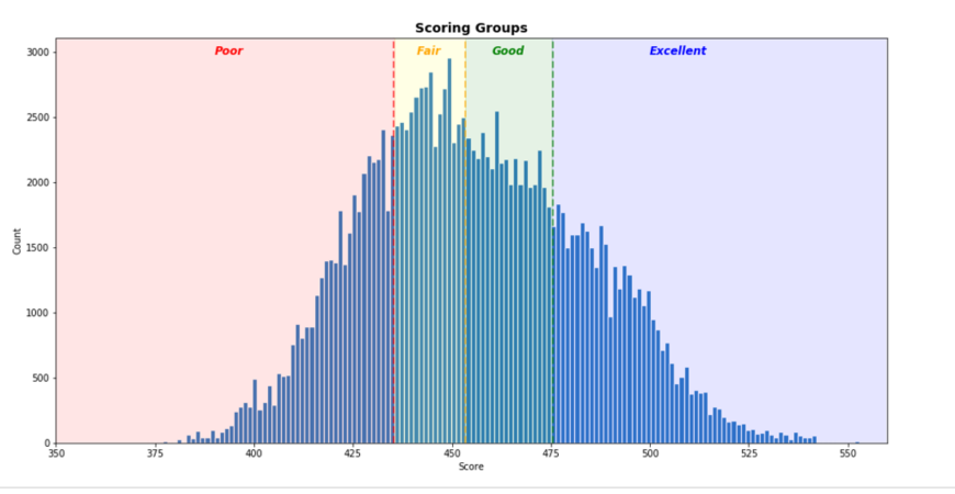
Finally, we can use those scores to determine tiers of consumers based on their credit score. Depending on the product, loan, etc. there will be varying bands for these tiers. For my tiering system I just selected quartiles to illustrate the building of cutoffs, but you could select any variation with a variety by product or offering.
Rejection inference
I want to briefly mention rejection inference, since it is an important step in credit scoring. To this point we’ve fit a logistic regression model based on a label of good or bad and scaled those scores into a scorecard. This entire process has looked at the current customer base which has mostly complete data and known credit (good or bad). However, applications for credit can often be missing a lot of data, which leads to a denial of credit. Denial of credit in this case is due to our biased model that only looks at complete records of people we know to be good or bad. We need to include some method to investigate the denials and include that information back into our model, so it is less bias and generalizes better.
This is what rejection inference achieves. In short, we look at those rejected customers, who have unknown credit status, and treat that data separately while then re-classifying them as good or bad. This is often achieved by rule-based approaches, proportional assignment similar to original logit model, augmenting original scores from logit for the denials, etc. This topic could be a standalone discussion since there are a variety of methods as well as schools of thought. For now, I’ll just state that to optimize your model to be unbiased and generalize better the denials, due to missing data, should be investigated and incorporated.
Summary
Overall, using weight of evidence transformations and a logistic regression model to derive scores for customers can be a very powerful tool in the hands of a data scientist who also uses logical sense of the business. There are many ways to build these scoring models and while this is just one I hope it’s helpful in giving guidance or spurring new ideas. Plus, any time a data scientist can take complex problems, like transformations and credit scoring, and illustrate the results it’s a win for both the practitioner and the organization.
Bonus: Scoring function or Rest API
I created a function that used the code parameter from our transformation and logistic regression to score new incoming data in batch. It can save time and show how to use your code for scoring new data.
Looking at Figure 12, the first step is generating a small test set and I do this by grabbing a couple observations from the training data (just for testing purposes). Then load that data to the CAS server. Here you can see the function I built called model_scoring. It takes 5 parameters: name of CAS connection, code from woe transformation, code from logistic regression model, test table name and the scored table name. If you look within the model_scoring function there are three steps:
- runcodetable - woe transform.
- impute – replace missing woe values with 0.
- runcodetable – logistic regression using woe transform values.
I use that scoring function to score the new data. At this point you would apply those simple scorecard calculations however you want to scale, and you would have a ready to use scorecard.

All of this can also be done using REST API’s. Every analytic asset on CAS is abstracted using a REST end point. This means that your data and your data processes are just a few REST calls away. This allows for easy integration of SAS technology into your business process or other applications. I accessed these action sets and actions using python, but with REST you can access any of these assets in the language of your choice.
References
- Siddiqi, Naeem. Credit Risk Scorecards: Developing and Implementing Intelligent Credit Scoring. 1st ed., Wiley, 2005.
- SAS Developer of ‘dataPreProcess’ Action Set and Huge Thanks to Biruk Gebremariam
- Full Jupyter Notebook demo on GitHub
- Additional Thanks: Wayne Thompson


2 Comments
Excellent article. Thanks for explaining how to transform probability into a score. Can you please help with your inputs on the below?
1. If I need a score between 1 - 100, what should I change? The target score?
2. With the target score of 600 in your example, how to calculate the minimum and maximum score (the score range)
Hi Andre,
Thanks a lot for your sharing, it's a very useful guide !
I have several questions.
1) Why do you use forward selection method for variable selection, is it better than stepwise selection in your experience?
2) The IV of age is greater than 0.7, in the book of Siddiqi, Naeem. Credit Risk Scorecards, said :"Characteristics with IV greater than 0.5 should be checked for overpredicting" , is there a potential
issue for over fitting?
3) It seems that SAS credit scoring use Fuzzy as default method for reject inference, could you have a brief introduce for it in Python, may be in another technical blog 🙂
Thanks,
Jidong