Improving model interpretability with LIME

We have updated our software for improved interpretability since this post was written. For the latest on this topic, read our new series on model-agnostic interpretability.

While some machine learning models – like decision trees – are transparent, the majority of models used today – like deep neural networks, random forests, gradient boosting machines, and ensemble models – are black-box models.

The interpretability of a machine learning model is essential for gaining insight into model behavior. Understanding the rationale behind the model's predictions would certainly help users decide when to trust or not to trust their predictions which is fundamental if one plans to take action based on a prediction, or when choosing whether to deploy a new model.

Local Interpretable Model-Agnostic Explanation (LIME) is an algorithm that provides a novel technique for explaining the outcome of any predictive model in an interpretable and faithful manner. It works by training an interpretable model locally around a prediction you want to explain.

The LIME technique was first developed by Marco Tulio Ribeiro, Sameer Singh, and Carlos Guestrin and described in the paper "Why Should I Trust You? Explaining the Predictions of Any Classifier." I use examples from their paper below to further introduce LIME and how it works.

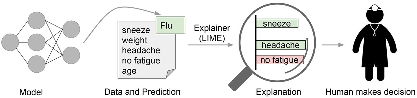
The first example, shown in Figure 1, illustrates a model that predicts whether a certain patient has the flu. The prediction is then explained by an "explainer" that highlights the symptoms that are most important to the model.

After all, a doctor is better positioned to make a decision with the help of a model if intelligible explanations are provided. In this case, an explanation is a small list of symptoms with relative weights - symptoms that either contribute to the prediction (in green - positive weight) or are evidence against it (in red - negative weight).

Figure 1. Explaining individual predictions to a human decision-maker. Source: KDD, Ribeiro, Singh, and Guestrin

Scope of interpretability

To better understand how LIME works, let's consider two distinct types of interpretability:

Global interpretability: Global interpretations help us understand the entire conditional distribution modeled by the trained response function, but global interpretations can be approximate or based on averages.
Local interpretability: Local interpretations promote understanding of a single data point or of a small region of the distribution, such as a cluster of input records and their corresponding predictions, or decile of predictions and their corresponding input rows. Because small sections of the conditional distribution are more likely to be linear, local explanations can be more accurate than global explanations.

LIME is designed to provide local interpretability, so it is most accurate for a specific decision or result.

Intuition behind LIME

We want the explainer to be model-agnostic and locally faithful. Locally faithful explanations capture the classifier behavior in the neighborhood of the instance to be explained. To learn a local explanation, LIME approximates the classifier's decision boundary around a specific instance using an interpretable model. LIME is model-agnostic, which means it considers the model to be a black-box and makes no assumptions about the model behavior. This makes LIME applicable to any predictive model.

In order to learn the behavior of the underlying model, LIME perturbs the inputs and sees how the predictions change. The key intuition behind LIME is that it is much easier to approximate a black-box model by a simple model locally than by a single global model. This is done by weighting the perturbed sample instances by their similarity to the instance we want to explain, fitting a Lasso model to select K features, and finally learning the K coefficients via linear regression.

This example is also from the Ribeiro, Singh, and Guestrin paper.

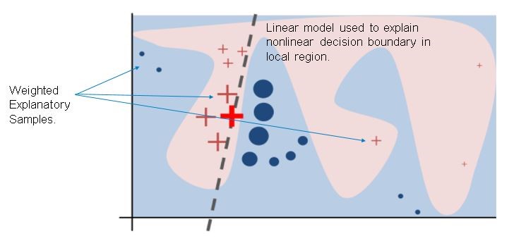
Figure 2: Presenting intuition for LIME. (Source: Ribeiro, Singh, and Guestrin)

The black-box model’s complex train function f (unknown to LIME) is represented by the blue/pink background, which cannot be approximated well by a linear model. The bold red cross is the instance being explained. LIME samples instances, gets prediction using f, and weights them by the proximity to the instance being explained (represented here by size). The dashed line is the learned explanation that is locally (but not globally) faithful.

Using LIME with SAS

The diagram below illustrates the general steps of the LIME technique implemented with SAS Visual Data Mining and Machine Learning. Note that the input can be any observation for which you want to provide an explanation. In the current version of the Model Studio application in SAS, clusters are generated from the training data and the cluster centroids are used as the to provide local model explanations for those clusters; for any new observation, the explanation can be attributed to the explanation for the cluster it is most closely associated with. In an upcoming release, a CAS action is being provided to allow for the explanations to be generated for any individual observation.

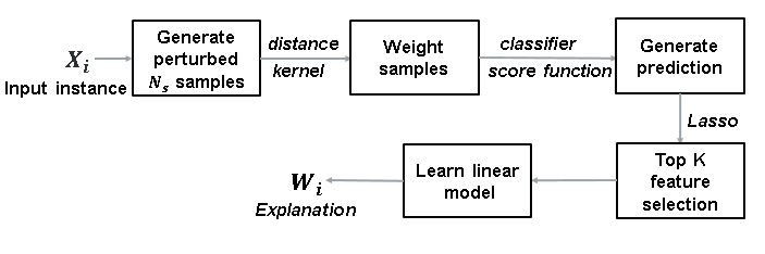
Figure 3: Functional block diagram of LIME generating an explanation for the prediction of the instance . The user may repeat the process N times. The final explanation is the average of the coefficients of the linear models over the N iterations.

Image example for LIME

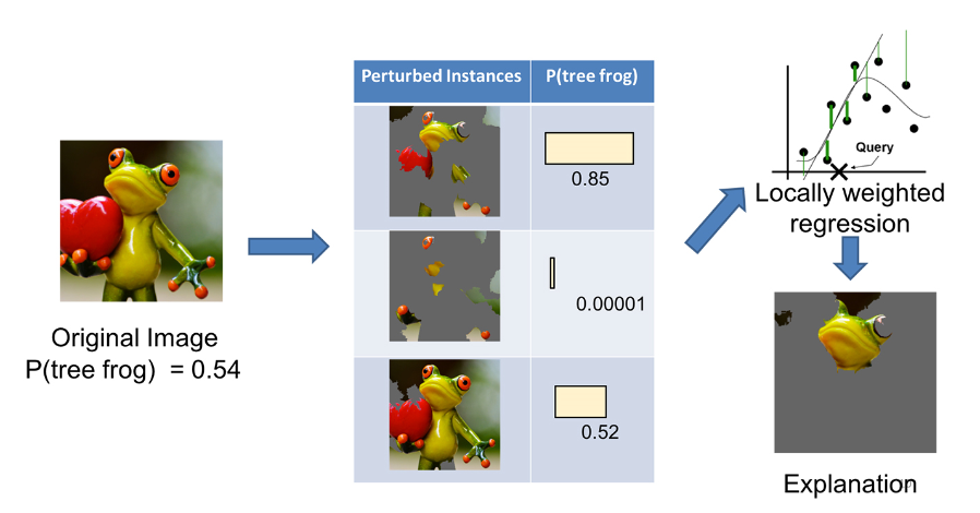
Another popular example of how LIME works for image classification is shown in Figure 4, in which we want to explain a classifier that predicts how likely it is for the image to contain a tree frog.

A data set of perturbed instances is generated by turning some of the interpretable pixels off (making them grey) in each image. Given an image whose prediction is to be explained, LIME generates a set of perturbed instances. For each perturbed instance, a prediction that a tree frog is in the image is computed using the black-box model.

A weighted LASSO regression is run on the perturbed instances, using the prediction from the black-box model as the target. In this example, the features are pixels. LASSO selects K of them. These are then used in a simple linear weighted regression on the same instances, weights, and target. In the end, the pixels with the highest positive coefficients serve as an explanation. The explanation is presented by showing the original image with the non-explaining pixels set to grey.

This example is from a second article by by Marco Tulio Ribeiro, Sameer Singh, and Carlos Guestrin, “Introduction to Local Interpretable Model-Agnostic Explanations (LIME),” published in O’Reilly.

Figure 4. An illustration of the LIME process in which a weighted linear model is used to explain a single prediction from a neural network. (Sources: Marco Tulio Ribeiro)

LIME use cases with SAS

Diabetes model explanations

Now I’ll show two simple use cases that illustrate the use of LIME on a SAS model, and how LIME improves interpretability of the model.

These examples use a SAS macro to provide an explanation for an individual observation (as opposed to the clustering approach used in Model Studio). This capability for individual explanations will be offered in an upcoming release, both as a CAS action and in Model Studio.

The first example uses a diabetes dataset available from UCI Machine Learning Repository. This is the well-known Akimel O’otham (formerly known as Pima Indians) diabetes dataset. A population of women who were at least 21 years old, of Akimel O’otham heritage and living near Phoenix, Arizona, was tested for diabetes according to World Health Organization criteria. The data were collected by the US National Institute of Diabetes and Digestive and Kidney Diseases.

We train a SAS neural network model on this data, which consists of 768 observations with the following variables:

A binary target: onset of diabetes
Eight interval features: number of times pregnant, plasma glucose, diastolic blood pressure, triceps skin fold thickness, 2-hour serum insulin, body mass index, diabetes pedigree function, and age.

To explain the prediction, LIME first looks at a diabetic woman of 50 years of age with a body mass index 33.6, diastolic blood pressure 72, triceps skin fold thickness 35mm, 2-hour serum insulin 0 mu U/ml, plasma glucose 148, number pregnancies 6 times, and diabetes pedigree function 0.627. The neural network model predicts the probability of this individual having diabetes to be 60%.

The results below show the local vs. global explanations for the diabetes model.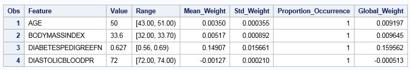

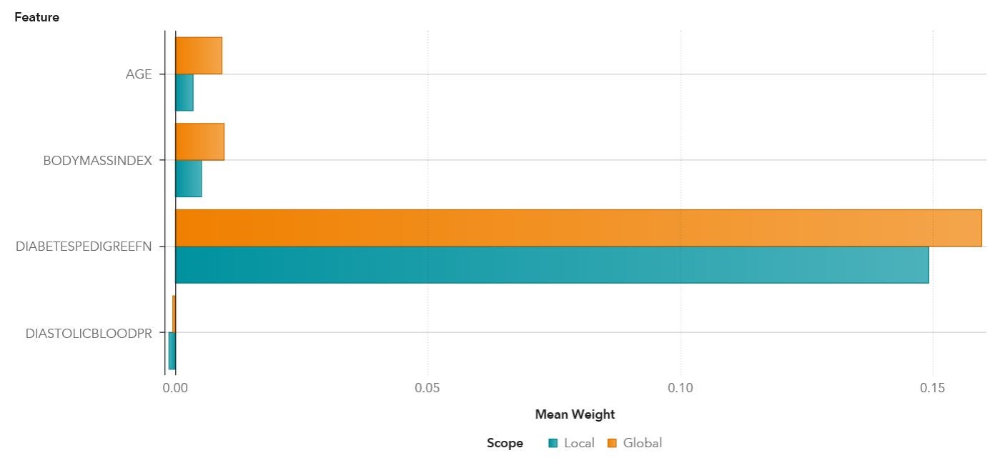
**Figure 8:** 1000 sample instances were generated using decile discretizer in each of 5 iterations, and weighted by a kernel function applying the distance computed by k prototype distance metric. Mean_Weight, Std_Weight presented in the results are the average and standard deviation of the coefficients of linear regression models trained on the top 4 features selected by LASSO penalized regression.

Age, body mass index, and diabetes pedigree function are linearly associated with increases in the probability of the onset of diabetes in both local and global explanations. By far, diabetes pedigree function is the most influential factor. When diabetes pedigree function measurement increases by 1 unit, the probability of predicting the individual having diabetes increases by 15% in the local explanation and 16% in the global explanation.

NBA players model explanations

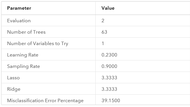
The second use case uses NBA Box Score Players Stats provided by Sportradar US LLC. We train a SAS gradient boosting model on this data consisting of 174194 records, including:

A binary target: shot_made_flag,
Eight interval inputs: age, heightInches, minutes_remaining, period, seconds_remaining, shot_distance, weightLbs, yrsExperience,
Three nominal inputs: position, shot_zone_area, and shot_zone_range

**Figure 9:** Gradient boosting autotuned best parameters

The case used to explain the model with LIME is the prediction of playerID 1495, age 40, height 83 inches, weigh 250 lbs, shot_made_flag=1, position is center-forward, shot_zone_area is fenter, shot_zone_range is less than 8ft. The player made the shot, and the prediction of the shot_made_flag1 = 0.6557.

The results below show the local versus global explanations for the NBA players model.

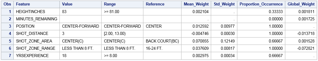
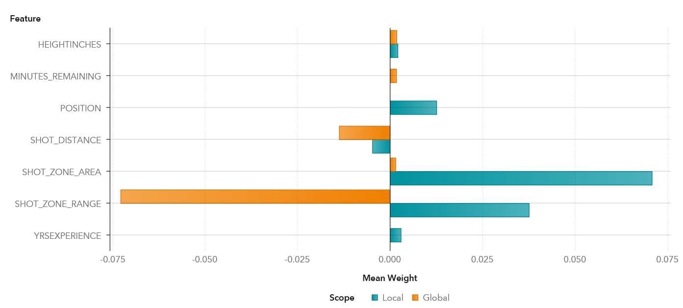
**Figure 10:** Perturbed 1000 sample instances were generated using quartile discretizer in each three iterations, and weighted by a kernel function applying the distance computed by cosine distance metric. Mean_Weight, Std_Weight presented in the results are the average and standard deviation of the coefficients of linear regression models trained on the top 5 features selected from LASSO penalized regression.

With a player of 83 inches in height, if the height increases by 1 inch, the probability of shot_ made_flag1 increases by 0.21%, which is similar to the global increase of 0.18%.

With a player who has 18 years of experience, for every extra year of experience, the probability of shot_ made_flag1 increases by 0.3%. However the years of experience is not one of the top five features selected from the global model.

Other features such as position, shot_zone_area, and shot_zone_range are nominal features.

For this player, comparing his shot_zone_area of “Center” with “Back Court,” the probability of shot_ made_flag1 is 7.1% greater than when shot_zone_area is “Back Court.” There is less difference on the global explanation, which only increases by 0.15%.

For shot_zone_range, comparing the player’s shot_zone_range of “less than 8 ft” with “16-24 ft”, the probability of shot_ made_flag1 increases by 3.76% over when shot_zone_range is 16-24 ft. In contrast, the global difference decreases by 7.28%.

Conclusion

Interpretability of black box models is overdue. LIME approaches the problem by fitting a linear model around a point to be interpreted, and then uses the coefficients of the surrogate model for interpretation. For SAS, LIME is just a beginning. We are actively researching other ideas to improve the interpretability of our models. More information will be announced in future blog posts.

Watch the webinar: Implementing AI Systems with Interpretability, Transparency and Trust

References: