Sequence models, especially recurrent neural network (RNN) and similar variants, have gained tremendous popularity over the last few years because of their unparalleled ability to handle unstructured sequential data. The reason these models are called “recurrent” is that they work with data that occurs in a sequence, such as text data and time stamped data. In this blog post, I’ll be focusing on text data as an example. I hope to write more blog posts about other interesting applications using an RNN later, so tell me the applications you want to see discussed next in the comments.
Since most machine learning models are unable to handle text data, and text data is ubiquitous in modern analytics, it is essential to have an RNN in your machine learning toolbox. RNNs excel at natural language understanding and how language generation works, including semantic analysis, translation, voice to text, sentiment classification, natural language generation and image captioning. For example, a chatbot for customer service must first understand the request of a customer, using natural language understanding techniques, then either route the request to the correct human responders, or use the natural language generation techniques to generate replies as naturally as possible.
RNN models are good at modeling text data because they can identify and “remember” important words in a sentence easily, such as entities, verbs, and strong adjectives. The unique structure of RNNs evaluate the words in a sentences one-by-one, usually from the beginning to the end. It uses the meaning of the previous word to infer the meaning of the next word or to predict the most likely next word.
Extracting sentiment with RNNs
Let’s briefly talk about the structure of RNNs using a very simple example. Suppose we want to build a model to extract the sentiment of customer reviews on Yelp. In this case, the training data set is manually labeled, “customer review text data set.” One of the customer reviews in the data set is,
“Friendly bartenders and a beautiful view.”
This sentence has six words and it is obviously positive. RNNs parse the training data as: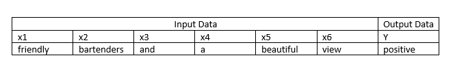
The diagram below shows the processing flow for the example sentence. \(h_0\) contains a set of initial values of parameters that will be updated step-by-step. \({A}\) represents parameters inside a hidden node, such as weights and biases. \(x_1\), which is vector representation of the word “friendly” and \(h_0\) together are used to calculate \(h_1\), \(x_2\) and \(h_1\) together are used to calculate \(h_2\), ... and so on. In the last step, the result of \(h_6\) is mapped to binary output (positive, negative). We will cover the details of the process later.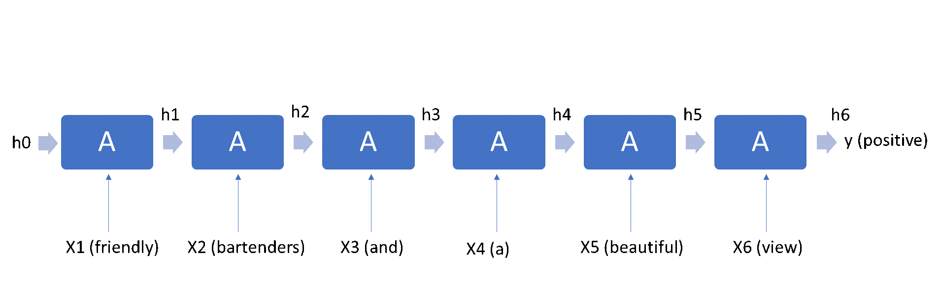
Note that the customer review data set likely contains many reviews written by different people. The review in the example above contains 6 words, but other reviews could contain fewer (or more) words. An RNN can analyze varying length input which is an advantage over traditional neural networks and other machine learning models.
Sentiment classification is a typical “many-to-one” problem, since there are many inputs (words in a sentence), but only one output (the sentiment). RNN can also handle other types of problems, such as one-to-one, one-to-many, and many-to-many. For example, translation is a many-to-many problem that translates many words in a language to many words in another language.
A basic RNN structure
Next let’s look at what is inside the RNN hidden neurons, in other words, the \(h_i\) and \({A}\). As we’ve stated, there are many types of RNN. For this example, let’s start from the simplest form.
In the simplest case, \(h_i\) is a set of parameters which only contain cell state information. Hidden neuron \({A}\) contains weights, \(W_h\) and \(W_x\), and a bias term \(b_h\). The weights and forward propagation is conducted first in order to determine the error signal at the output of the network, then the weights/biases are updated using back propagation. Also, RNNs typically use a special form of backpropagation called “backpropagation through time” (BPTT). Please note that the weights and biases are the same in every step, and that is part of the reason the model is called recurrent. \(h_t\) is updated by the following equation in each hidden neuron \({A}\). The " \(\cdot\) " here means matrix multiplication. " * " in later equations means element-wise multiplication.
\(h_t = tanh(W_h \cdot h_{t-1} + W_x \cdot x_t + b_h)\)
In the example of sentiment analysis, there is only one output from a sequence, the sentiment class, \(y\). Its probability distribution is calculated by a sigmoid function based on the final cell state, \(h_t\).
\(y_{pred} = sigmoid(W_y \cdot h_t + b_y)\)
A major drawback in a basic RNN occurs when the sequence is very long, which causes problems of exploding gradients and vanishing gradients. I’m not going to talk about technical details of those problems here, but they make the numerical optimization very slow and very inaccurate, and sometimes do not even converge. Since the Yelp reviews include many long sequences of text, we will use a gated RNN in our analysis.
Gated recurrent unit
A gated recurrent unit is a popular variation of RNN. It has a simple structure and is easy to tune and use. It is much better than the basic form in handling long term memories and small data sets. The only modification it makes on a basic RNN is adding two “gates” to the previous basic RNN structure, an “update” gate, \(u_t\) and a “reset” gate, \(r_t\).
The “gates” essentially control how much previous information is used in the current hidden neuron. For example, they might ignore unimportant words like “a” and “the” from carrying through for analysis. Or they can put more weight on words that carry more value for sentiment. Their values are continuous between 0 and 1.
The reset gate, \(r_t\) controls how much the previous state \(h_{t-1}\) influences the candidate state \(\tilde{h}_{t}\). Should \(r_t\) fall to zero, the GRU candidate state is reset to the next sequence input. The update gate, \(u_t\) controls how much the candidate state \(\tilde{h}_{t}\) influences the next state \(h_t\). When the update falls to zero, the previous state is used as the current state. Similarly, when update is one, then the candidate state is used as the next state. The two gates controls RNN via the following equations.
\(\tilde{h}_{t} = tanh(W_h \cdot r_t \cdot h_{t-1} + W_x \cdot x_t + b_h )\)
\(h_t = u_t * h_{t-1} + (1-u_t) * \tilde{h}_{t}\)
The two gates are calculated by the following two equations.
\(u_t = sigmoid(W_u\cdot[h_{t-1},x_t] + b_u)\)
\(r_t = sigmoid(W_r\cdot[h_{t-1},x_t] + b_r)\)
The output y is calculated in the same way as simple RNN. In the case of sentiment analysis, the probability distribution of the sentiment class, \(y\) is calculated by a sigmoid function based on the final cell state, \(h_t\).
\(y_{pred} = sigmoid(W_y \cdot h_t + b_y)\)
Long short-term memory
The long short-term memory model (LSTM) has one more gate than GRU. GRU only has two gates, while LSTM has three gates: the forget gate, input gate and output gate. LSTM splits the update gate in GRU to forget gate and input gate, and replaces the reset gate by output gate.
LSTM has a more complicated structure, thus it’s more flexible than GRU. It usually takes a longer time in tuning. The gates are calculated using the following equations. Please note that these equations are without “peephole” connections. Some practitioners prefer a LSTM variant with “peephole” connections, which add cell states information to all or some of the sigmoid functions in the following equations.
\(i_t = sigmoid(W_i\cdot[h_{t-1},x_t] + b_i)\)
\(o_t = sigmoid(W_o\cdot[h_{t-1},x_t] + b_o)\)
\(f_t = sigmoid(W_f\cdot[h_{t-1},x_t] + b_f)\)
Because of the additional forget gate, LSTM splits the cell state into two sequences \(C_t\) and \(h_t\) The following diagram describes how the example review, “Friendly bartenders and a beautiful view” works in LSTM.
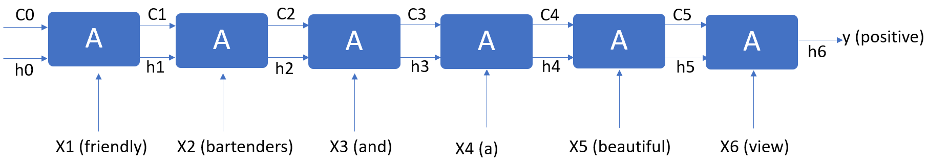
\(C_t\) represents the current cell state while \(h_t\) is the current cell activation. Here is how \(C_t\) and \(h_t\) are updated.
\(\tilde{C}_{t} = tanh(W_h \cdot h_{t-1} + W_x \cdot x_t + b_c )\)
\(C_t = i_t * \tilde{C}_{t} + f_t * C_{t-1}\)
\(h_t = o_t * tanh(C_t)\)
The output \(y\) is calculated in the same way as simplest RNN. In the case of sentiment analysis, the probability distribution of the sentiment class, \(y\) is calculated by a sigmoid function based on the final cell state, \(h_t\).
\(y_{pred} = sigmoid(W_y \cdot h_t + b_y)\)
Please note that LSTM was proposed much earlier than GRU. The only reason we introduce GRU before LSTM is that GRU is easier to understand for beginners.
Real data example
Finally, let’s see a real example using GRU to detect sentiment in Yelp reviews. This example uses Python code for the GRU model but SAS Viya also supports R, Java, Lua and, of course, SAS code. You can find the entire notebook in Github. There is also an R version here. In the blog, I am going to focus on only the most relevant code snippet – defining the RNN model architecture.
In this example, a GRU model is used as specified by the option "rnnType." Other RNN layer types "LSTM" and "RNN" are available.
In layers rnn11 and rnn21, reverse = True is specified, and that makes the GRU bi-directional. Specifically, layers rnn11 and rnn21 are in the reverse direction, which means the model scans the sentence from the end to the beginning, while rnn12 and rnn22 are in the common forward direction. Therefore, the state of a neuron is not only affected by the previous words, but also the words after the neuron.
# Sentiment classification # In this example, GRU model is used as specified by the option "rnnType". You can specify other layer types "LSTM" and "RNN". # In some layers, reverse = True is specified, and that makes GRU bi-directional. Specifically, layers rnn11 and rnn 21 # are in the reverse direction, which means the model scan the sentence from the end to the beginning, while rnn12 and rnn22 are # in the common forward direction. Therefore, the state of a neuron is not only affected by the previous words, but also the # words after the neuron. n=64 init='msra' s.buildmodel(model=dict(name='sentiment', replace=True), type='RNN') s.addlayer(model='sentiment', name='data', layer=dict(type='input')) s.addlayer(model='sentiment', name='rnn11', srclayers=['data'], layer=dict(type='recurrent',n=n,init=init,rnnType='GRU',outputType='samelength', reverse=True)) s.addlayer(model='sentiment', name='rnn12', srclayers=['data'], layer=dict(type='recurrent',n=n,init=init,rnnType='GRU',outputType='samelength', reverse=False)) s.addlayer(model='sentiment', name='rnn21', srclayers=['rnn11', 'rnn12'], layer=dict(type='recurrent',n=n,init=init,rnnType='GRU',outputType='samelength', reverse=True)) s.addlayer(model='sentiment', name='rnn22', srclayers=['rnn11', 'rnn12'], layer=dict(type='recurrent',n=n,init=init,rnnType='GRU',outputType='samelength', reverse=False)) s.addlayer(model='sentiment', name='rnn3', srclayers=['rnn21', 'rnn22'], layer=dict(type='recurrent',n=n,init=init,rnnType='GRU',outputType='encoding')) s.addlayer(model='sentiment', name='outlayer', srclayers=['rnn3'], layer=dict(type='output')) |
To learn more about RNNs, check out The SAS Deep Learning Python (DLPy) package on github or explore the SAS Deep Learning documentation.
Thank you to Doug Cairns for his tremendous help in the technical review and editing of this blog post.


1 Comment
Thanks for this very nice writeup and the notebook. I would love to learn from you how RNN treats time series data especially if they are not stationary.