Learning never stops. When SAS had to change this year’s SAS Global Forum (SASGF) to a virtual event, everyone was disappointed. I am, however, super excited about all of the papers and stream of video releases over the last month (and I encourage you to register for the upcoming live event in June). For now, I made a pact with myself to read or watch one piece of SASGF related material per day. While I haven’t hit my goal 100%, I sure have learned a lot from all the reading and viewing. One particular paper, Using Jupyter to Boost Your Data Science Workflow, and its accompanying SASGF video by Hunter Glanz caught my eye this week. Also, be sure to check out Hunter's How To Tutorial video on this topic. Both videos appear on the SASUsers YouTube Channel. This post elaborates on one piece of his material: how to save Jupyter notebooks in other file formats.
Hunter’s story
Hunter is a professor who teaches multiple classes using SAS® OnDemand for Academics, which comes equipped with an integrated Jupyter notebook. His focus is on SAS programming and he requires his students to create notebooks to complete assignments; however he wants to see the results of their work, not to run their raw code. The notebooks include text, code, images, reports, etc. Let's explore how the students can transform their navitve notebooks into other, more consumable formats. We'll also discuss other use cases in which SAS users may want to create a copy of their work from a notebook, to say a .pdf, .html, or .py file, just to name a few.
What you’ll find here and what you won’t
Many of the processes discussed below are language agnostic. When there are distinct differences, I’ll make a note.
A LITTLE about Jupyter notebooks
A Jupyter notebook is a web application allowing clients to run commands, view responses, include images, and write inline text all in one concourse. The all-encompassing notebook supports users to telling complete story without having to use multiple apps. Jupyter notebooks were originally created for the Python language, and are now available for many other programming languages. JupyterLab, the notebooks’ cousin, is a later, more sophisticated version, but for this writing, we’ll focus on the notebook. The functionality in this use case is similar.
Where do we start? First, we need to install the notebook, if you're not working in SAS OnDemand for Academics.
Install Anaconda
The easiest way to get started with the Jupyter Notebook App is by installing Anaconda (this will also install JupyterLab). Anaconda is an open source distribution tool for the management and deployment of scientific computing. Out-of-the-box, the notebook from the Anaconda install includes the Python kernel. For use with other languages, you need to install additional kernels.
Install additional language kernels
In this post, we’ll focus on Python, R, and SAS. The Python kernel is readily available after the Anaconda install. For the R language, follow the instructions on the GitHub R kernel repository. I also found the instructions on How to Install R in Jupyter with IRKernel in 3 Steps quite straight forward and useful. Further, here are the official install instructions for the SAS kernel and a supporting SAS Community Library article.
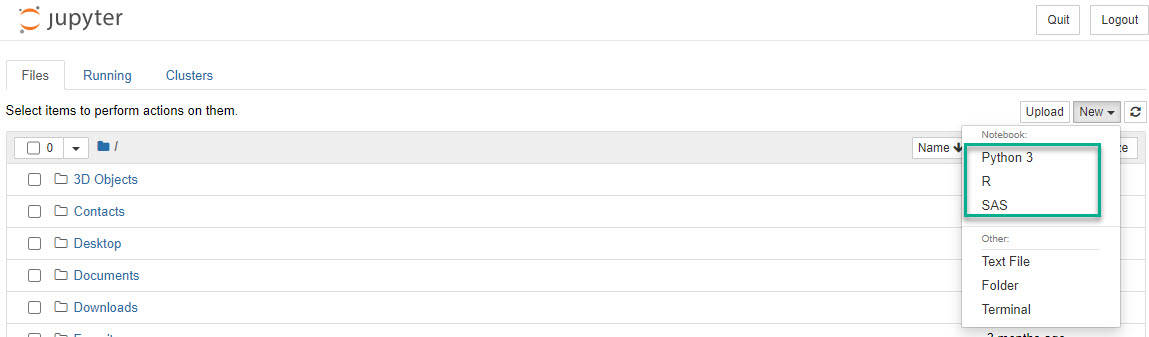
With the additional kernels are in place, you should see all available languages when creating a new notebook as pictured below.
File conversion methods
Now we’re ready to dive into the export process. Let’s look at three approaches in detail.
Download (Export) option
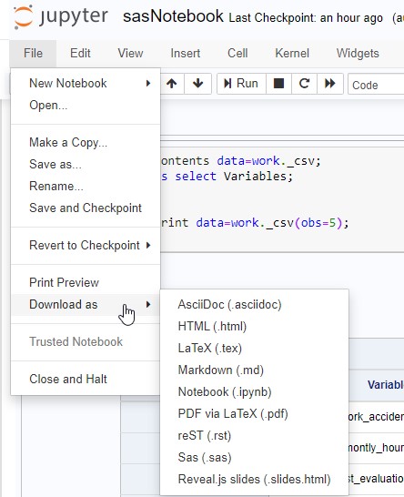
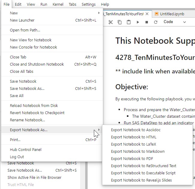
Once you’ve opened your notebook and run the code, select File-> Download As (appears as Export Notebook As… in JupyterLab).
HTML format output
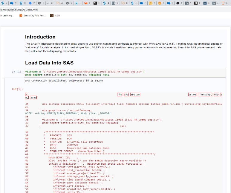
Notice the list of options, some more familiar than others. Select the HTML option and Jupyter converts your entire notebook: text, commands, figures, images, etc, into a file with a .html extension. Opening the resulting file would display in a browser as expected. See the images below for a comparison of the .ipynb and .html files.

SAS (aka script) format output
Using the Save As-> SAS option renders a .sas file and is depicted in Enterprise Guide below. Note: when using a different kernel, say Python or R, you have the option to save in that language specific script format.
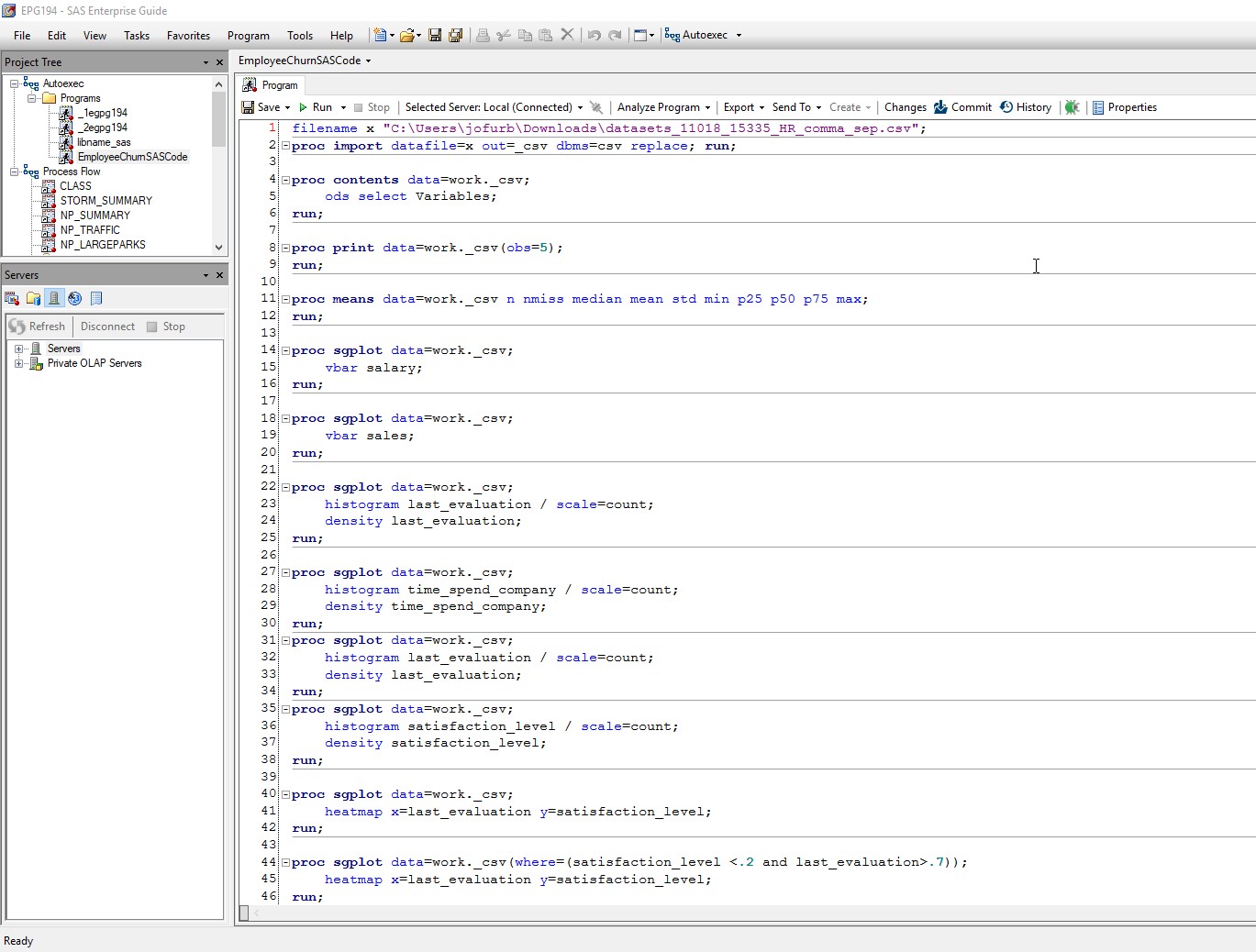
One thing to note here is only the code appears in the output file. The markdown code, figures, etc., from the original notebook, are not display options in EG, so they are removed.
PDF format output
There is one (two actually) special case(s) I need to mention. If you want to create a PDF (or LaTeX, which is used to create pdf files) output of your notebook, you need additional software. For converting to PDF, Jupyter uses the TeX document preparation ecosystem. If you attempt to download without TeX, the conversion fails, and you get a message to download TeX. Depending on your OS the TeX software will have a different name but will include TeX in the name. You may also, in certain instances, need Pandoc for certain formats. I suggest installing both to be safe. Install TeX from its dowload site. And do the same for Pandoc.
Once I’ve completed creating the files, the new files appear in my File Explorer.

Cheaters may never win, but they can create a PDF quickly
Well, now that we’ve covered how to properly convert and download a .pdf file, there may be an easier way. While in the notebook, press the Crtl + P keys. In the Print window, select the Save to PDF option, choose a file destination and save. It works, but I felt less accomplished afterward. Your choice.
Inline code option
Point-and-click is a perfectly valid option, but let’s say you want to introduce automation into your world. The jupyter nbconvert command provides the capability to transform the current notebook into any format mentioned earlier. All you must do is pass the command with a couple of parameters in the notebook.
In Python, the nbconvert command is part of the os library. The following lines are representative of the general structure.
import os os.system("jupyter nbconvert myNotebook.ipynb --to html") |
An example with Python
The example below is from a Python notebook. The "0" out code represents success.
An example with SAS
As you see with the Python example, the code is just that: Python. Generally, you cannot run Python code in a Jupyter notebook running the SAS kernel. Luckily we have Jupyter magics, which allow us to write and run Python code inside a SAS kernel. The magics are a two-way street and you can also run SAS code inside a Python shell. See the SASPy documentation for more information.
The code below is from a SAS notebook, but is running Python code (triggered by the %%python magic).
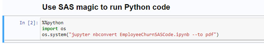
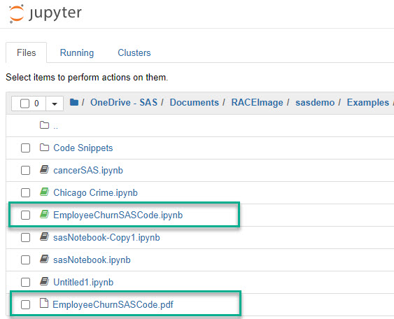
The EmployeeChurnSASCode.pdf file is created in same directory as the original notebook file:
An example with R
Things are fairly straight forward in an R notebook. However, you must install and load the nbconvert package.
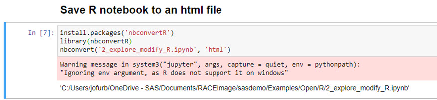
The first line installs the package, the second line loads the package, and the third actually does the conversion. Double-check your paths if you run into trouble.
The command line
The last method we look at is the command line. This option is the same regardless of the language with which you’re working. The possibilities are endless for this option. You could include it in a script, use it in code to run and display in a web app, or create the file and email it to a colleague. The examples below were all run on a Windows OS machine using the Anaconda command prompt.
An example with a SAS notebook
Convert sasNotebook.ipynb to a SAS file.
>> ls -la |grep sasNotebook -rw-r--r-- 1 jofurb 1049089 448185 May 29 14:34 sasNotebook.ipynb >> jupyter nbconvert --to script sasNotebook.ipynb [NbConvertApp] Converting notebook sasNotebook.ipynb to script [NbConvertApp] Writing 351 bytes to sasNotebook.sas >> ls -la |grep sasNotebook -rw-r--r-- 1 jofurb 1049089 448185 May 29 14:34 sasNotebook.ipynb -rw-r--r-- 1 jofurb 1049089 369 May 29 14:57 sasNotebook.sas |
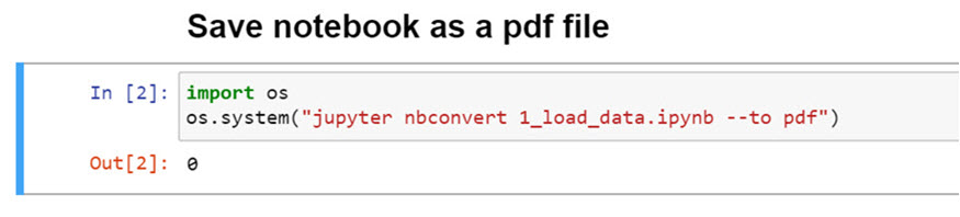
An example with a Python notebook
Convert 1_load_data.ipynb to a PDF file
>> ls -la |grep 1_load -rw-r--r-- 1 jofurb 1049089 6004 May 29 07:37 1_load_data.ipynb >> jupyter nbconvert 1_load_data.ipynb --to pdf [NbConvertApp] Converting notebook 1_load_data.ipynb to pdf [NbConvertApp] Writing 27341 bytes to .\notebook.tex [NbConvertApp] Building PDF [NbConvertApp] Running xelatex 3 times: ['xelatex', '.\\notebook.tex', '-quiet'] [NbConvertApp] Running bibtex 1 time: ['bibtex', '.\\notebook'] [NbConvertApp] WARNING | b had problems, most likely because there were no citations [NbConvertApp] PDF successfully created [NbConvertApp] Writing 32957 bytes to 1_load_data.pdf >> ls -la |grep 1_load -rw-r--r-- 1 jofurb 1049089 6004 May 29 07:37 1_load_data.ipynb -rw-r--r-- 1 jofurb 1049089 32957 May 29 15:23 1_load_data.pdf |
An example with an R notebook
Convert HR_R.ipynb to an R file.
>> ls -la | grep HR -rw-r--r-- 1 jofurb 1049089 5253 Nov 19 2019 HR_R.ipynb >> jupyter nbconvert HR_R.ipynb --to script [NbConvertApp] Converting notebook HR_R.ipynb to script [NbConvertApp] Writing 981 bytes to HR_R.r >> ls -la | grep HR -rw-r--r-- 1 jofurb 1049089 5253 Nov 19 2019 HR_R.ipynb -rw-r--r-- 1 jofurb 1049089 1021 May 29 15:44 HR_R.r |
Wrapping things up
Whether you’re a student of Hunter’s, an analyst creating a report, or a data scientist monitoring data streaming models, you may have the need/requirement to transform you work from Jupyter notebook to a more consumable asset. Regardless of the language of your notebook, you have multiple choices for saving your work including menu options, inline code, and from the command line. This is a great way to show off your creation in a very consumable mode.

1 Comment
Hello!
check out this SESUG.2021 paper on what one needs to know about using LaTeX (*.tex)
to create a pdf from Jupyter Notebook output.
https://www.lexjansen.com/sesug/2021/SESUG2021_Paper_8_Final_PDF.pdf
Ron Fehd macro maven