This article continues a series that began with Machine learning with SASPy: Exploring and preparing your data (part 1). Part 1 showed you how to explore data using SASPy with Python. Here, in part 2, you will learn how to begin to prepare your data to use it within a machine-learning model. 
Review part 1 if needed and ensure you still have the ADULT data set ready to use. (The data set is available from the UCI Machine Learning Repository.) If not, take some time to download and explore the data again, as described in part 1.
Preparing your data
Preparing data is a necessary step to perform before applying the data toward a model. There are string values, skewed data, and missing data points to consider. In the data set, be sure to clear missing values, so you can jump into other methods.
For this exercise, you will explore how to transform skewed features using SASPy and Pandas.
First, you must separate the income data from the data set, because the income feature will later become your target variable to model.
Drop the income data and turn the pandas data frame back into a SAS data object, with the following code:

![]()
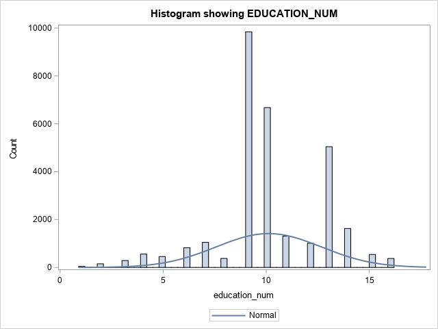
Now, let's take a second look at the numerical features. You will use SASPy to create a histogram of all numerical features. Typically, the Matplotlib library is used, but SASPy provides great opportunities to visualize the data.

The following graphs represent the expected output.
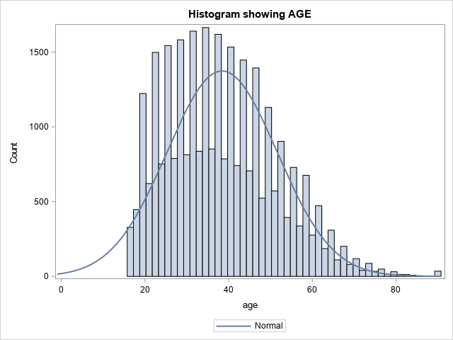
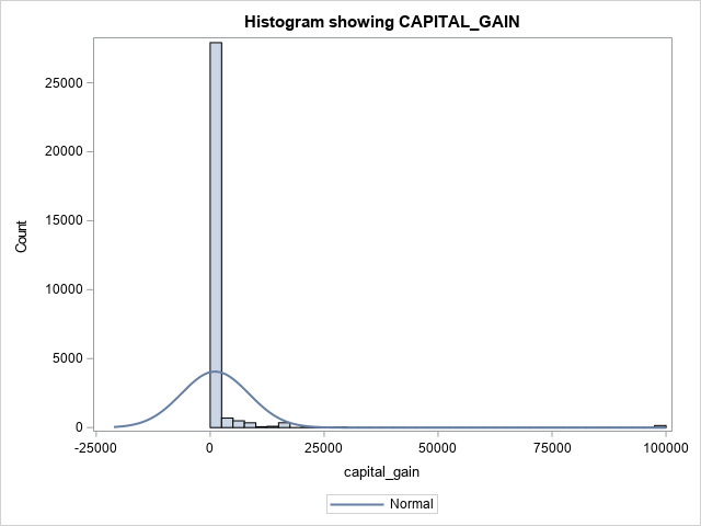
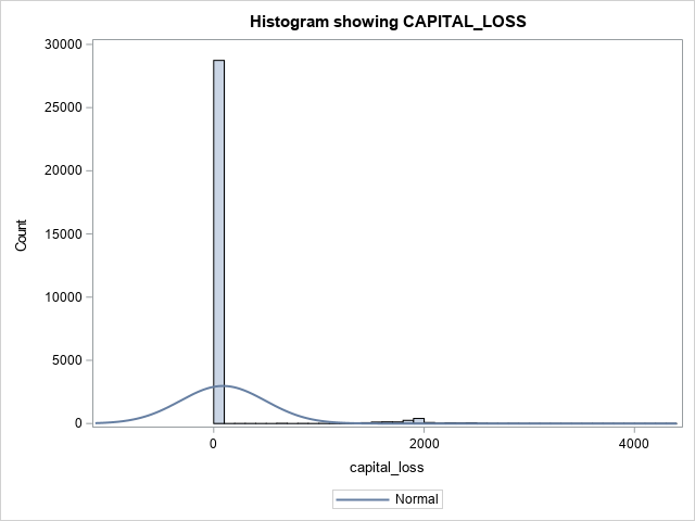
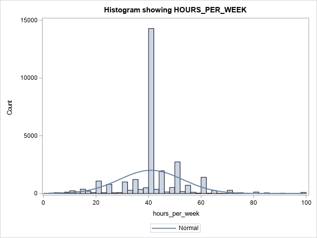
Taking a look at the numerical features, two values stick out. CAPITAL_GAIN and CAPITAL_LOSS are highly skewed. Highly skewed features can affect your model, as most models try to maintain a normally distributed curve. To fix this, you will apply a logarithmic transformation using pandas and then visualize the change using SASPy.
Transforming skewed features
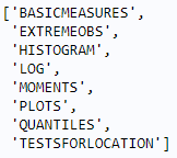
First, you need to change the SAS data object back into a pandas data frame and assign the skewed features to a list variable:
![]()
![]()
Then, use pandas to apply the logarithmic transformation and convert the pandas data frame back into a SAS data object:
![]()
![]()
Display transformed data
Now, you are ready to visualize these changes using SASPy. In the previous section, you used histograms to display the data. To display this transformation, you will use the SASPy SASUTIL class. Specifically, you will use a procedure typically used in SAS, the UNIVARIATE procedure.
To use the SASUTIL class with SASPy, you first need to create a Python object that uses the SASUTIL class:
![]()
Now, use the univariate function from SASPy:

Using the UNIVARIATE procedure, you can set axis limits to the output histograms so that you can see the data in a clearer format. After running the selected code, you can use the dir() function to verify successful submission:
![]()
Here is the output:
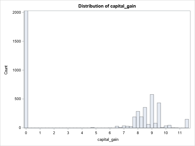
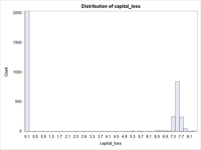
The function calculates various descriptive statistics and plots. However, for this example, the focus is on the histogram.
![]()
Here are the results:
Wrapping up
You have now transformed the skewed data. Pandas applied the logarithmic transformation and SASPy displayed the histograms.
Up next
In the next and final article of this series, you will continue preparing your data by normalizing numerical features and one-hot encoding categorical features.

1 Comment
If you want to know why the histogram of Age looks so bizarre, read "The mystery of the density curve that was too short."