SAS Visual Forecasting 8.2 effectively models and forecasts time series in large scale. It is built on SAS Viya and powered by SAS Cloud Analytic Services (CAS).
In this blog post, I will build a Visual Forecasting (VF) Pipeline, which is a process flow diagram whose nodes represent tasks in the VF Process. The objective is to show how to perform the full analytics life cycle with large volumes of data: from accessing data and assigning variable roles accurately, to building forecasting models, to select a champion model and overriding the system generated forecast. In this blog post I will use 1,337 time series related to a chemical company and will illustrate the main steps you would use for your own applications and datasets.
In future posts, I will work in the Programming application, a collection of SAS procedures and CAS actions for direct coding or access through tasks in SAS Studio, and will develop and assess VF models via Python code.
In a VF pipeline, teams can easily save forecast components to the Toolbox to later share in this collaborative environment.
Forecasting Node in Visual Analytics
This section briefly describes what is available in SAS Visual Analytics, the rest of the blog discusses SAS Visual Forecasting 8.2.
In SAS Visual Analytics the Forecast object will select the model that best fits the data out of these models: ARIMA, Damped trend exponential smoothing, Linear exponential smoothing, Seasonal exponential smoothing, Simple exponential smoothing, Winters method (additive), or Winters method (multiplicative). Currently there are no diagnostic statistics (MAPE, RMSE) for the model selected.
You can do “what-if analysis” using the Scenario Analysis and Goal Seeking functionalities. Scenario Analysis enables you to forecast hypothetical scenarios by specifying the future values for one or more underlying factors that contribute to the forecast. For example, if you forecast the profit of a company, and material cost is an underlying factor, then you might use scenario analysis to determine how the forecasted profit would change if the material cost increased by 10%. Goal Seeking enables you to specify a target value for your forecast measure, and then determine the values of underlying factors that would be required to achieve the target value. For example, if you forecast the profit of a company, and material cost is an underlying factor, then you might use Goal Seeking to determine what value for material cost would be required to achieve a 10% increase in profit.
Another neat feature in SAS Visual Analytics is that one can apply different filters to the final forecast. Filters are underlying factors or different levels of the hierarchy, and the resulting plot incorporates those filters.
Data Requirements for Forecasting
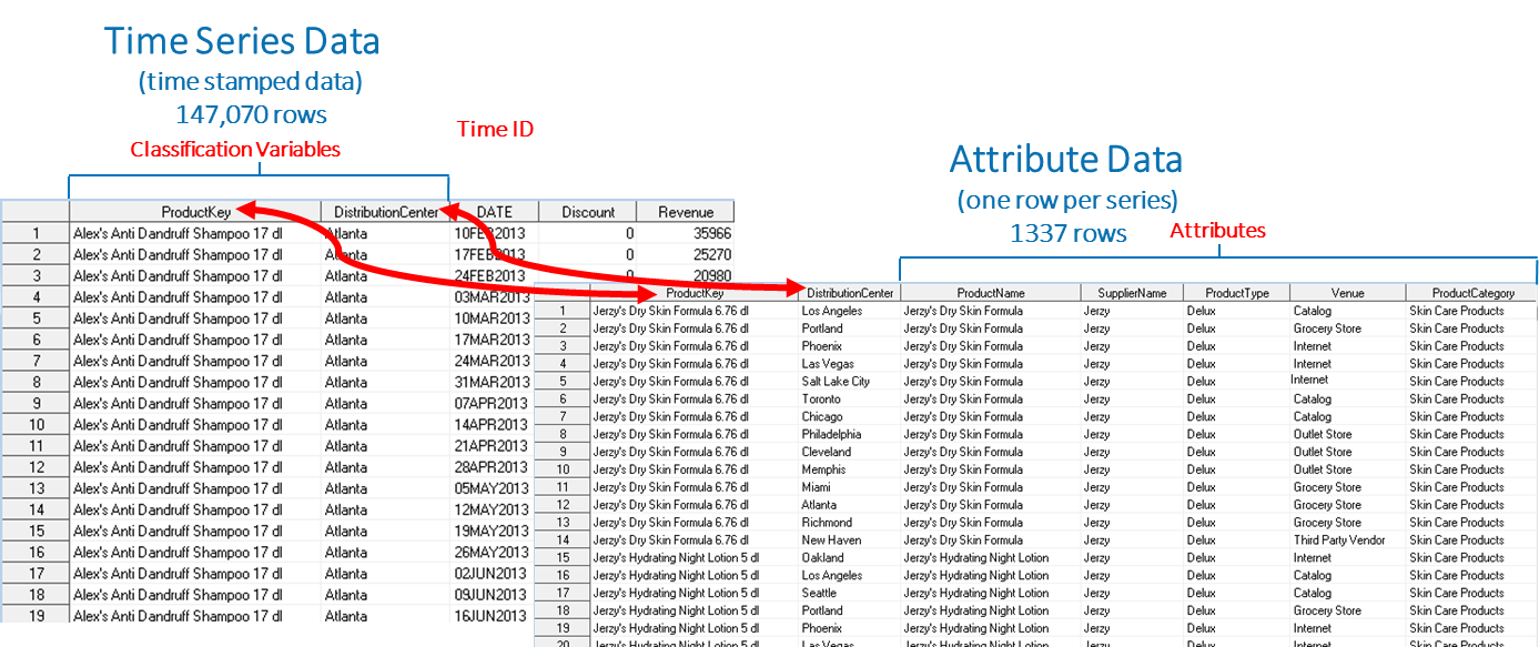
There are specific data requirements when working in a forecasting project, a time series dataset that contains at least two variables: 1) the variable that you want to forecast which is known as the target of your analysis, for example, Revenue and 2) a time ID variable that contains the time stamps of the target variable. The intervals of this variable are regularly spaced. Your time series table can contain other time-varying variables. When your time series table contains more than one individual series, you might have classification variables, as shown in the photo below. Distribution Center and Product Key are classification variables. Optionally, you can designate numerical variables (ex: Discount) as independent variables in your models.
You also have the option of adding a table of attributes to the time series table. Attributes are categorical variables that define qualities of the time series. Attribute variables are similar to BY variables, but are not used to identify the series that you want to forecast. In this post, the data I am using includes Distribution Center, Supplier Name, Product Type, Venue and Product Category. Notice that the attributes are time invariant, and that the attribute table is much smaller than the time series table.
The two data sets (SkinProduct and SkinProductAttributes) used in this blog contain 1,337 time series related to a chemical company. This picture shows a few rows of the two data sets used in this post, note that DATE intervals are regularly spaced weeks. The SkinProduct dataset is referred as the Time Series table in the SkinProductAttributes dataset as the Attribute Data.
Developing Models in SAS Visual Forecasting 8.2
Step One: Create a Forecasting Project and Assign Variables
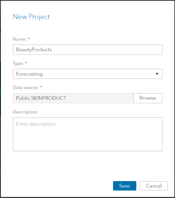
From the SAS Home menu select the action Build Models that will take you to SAS Model Studio, where you select New Project, and enter 1) the Name of your project, 2) the Type of project, make sure you enter “Forecasting” and 3) the data source.
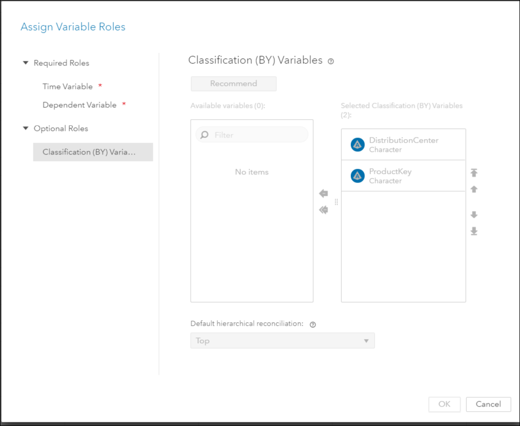
In the Data tab, assign the variables roles by using the icon in the upper right corner.
The roles assigned in this post are typical of role assignments in forecasting projects. Notice these variables are in the Time Series table. Also, notice that the classification variables are ordered from highest to lowest hierarchy:
Time Variable: Date
Dependent Variable: Revenue
Classification Variables: Distribution Center and Product Key
In the Time Series table, you might have additional variables you’d like to assign the role “independent” that should be considered for model generation. Independent variables are the explanatory, input, predictor, or causal variables that can be used to model and forecast the dependent variable. In this post, the variable “Discount” is assigned the role “independent”. To do this assignment: right click on the variable, and select Edit Variables.
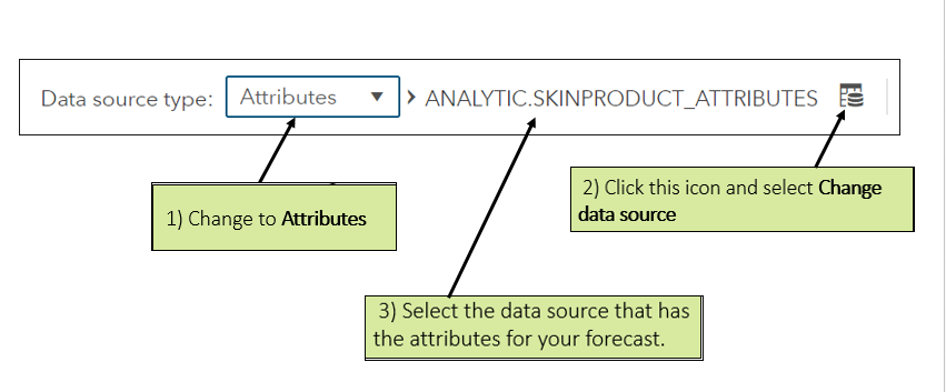
To bring in the second dataset with the Attribute variables, follow the steps in this photo:
Step two: Automated Modeling with Pipelines
The objective in this step is to select a champion model. Working in the Pipelines tab, one explores the time series plots, uses the code editor to modify the default model, adds a 2nd model to the pipeline, compares the models and selects a champion model.
After step one is completed, select the Pipelines Tab

The first node in the VF pipelines is the Data node. After right-clicking and running this node, one can see the time series by selecting Explore Time Series. Notice that one can filter by the attribute variables, and that the table shows the exact historical data values.
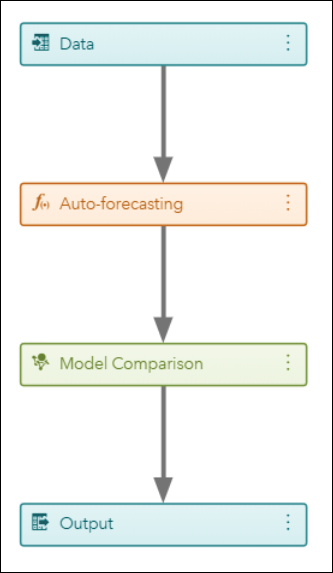
Auto-forecasting is the next node in the default pipeline. Remember that we are modeling 1,332 time series. For each time series, the Auto-forecasting node automatically diagnoses the statistical characteristics of the time series, generates a list of appropriate time series models, automatically selects the model, and generates forecasts. This node evaluates and selects for each time series the ARIMAX and exponential smoothing models.
One can customize and modify the forecasting models (except the Hierarchical Forecasting model) by editing the model’s code. For example, to add the class of models for intermittent demand to the auto- forecasting node, one could open the code editor for that node and replace these lines
rc = diagspec.setESM();
rc = diagspec.setARIMAX();
with:
rc = diagspec.setIDM();
To open the code editor see photo below. After changes, save code and close the editor.
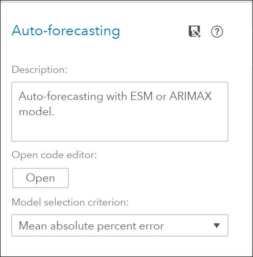
At this point, you can run the Auto Forecasting node, and after looking at its results, save it to the toolbox, so the editing changes are saved and later reused or shared with team members.
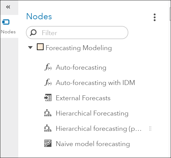
By expanding the Nodes pane and the Forecasting Modeling pane on the left, you can select from several models and add a 2nd modeling node to the pipeline
The next photo shows a pipeline with the Naïve Forecast as the second model. It was added to the pipeline by dropping its node into the parent node (data node). This is the resulting pipeline:
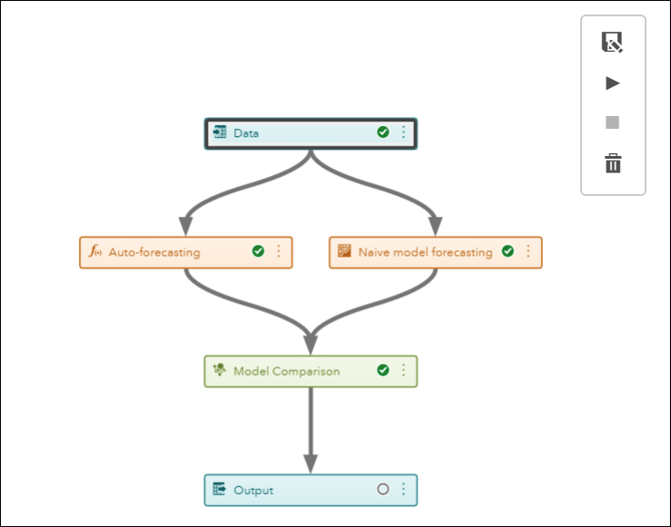
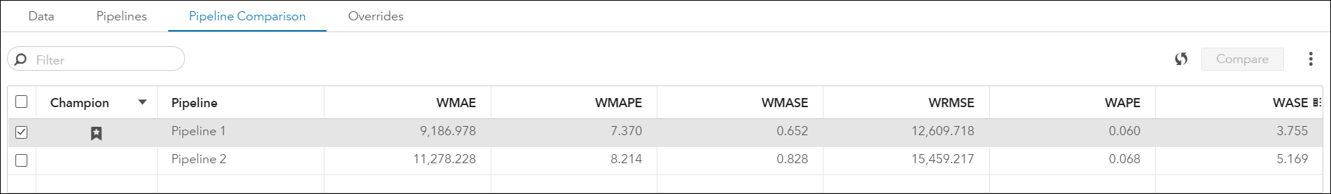
After running the Model Comparison node, compare the WMAE (Weighted Mean Absolute Error) and WMAPE (Weighted Mean Absolute Percent Error) and select a champion model.
You can build several pipelines using different model strategies. In order to select a champion model from all the models developed in the pipelines one uses the Pipeline Comparison tab.
![]()
Before you work on any overrides for your forecasting project, you need to make sure that you are working with the best pipeline and modeling node for your data. SAS Visual Forecasting selects the best fit model in each pipeline. After each pipeline is run, the champion pipeline is selected based on the statistics of fit that you chose for the selection criteria. If necessary, you can change the selected champion pipeline.
Step Three: Overrides
The Overrides tab is used to manually adjust the forecasts in the future. For example, if you want to account for some promotions that your company and its competitors are running and that are not captured by the models.
![]()
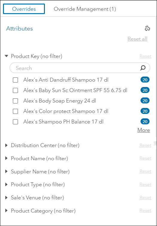
The Overrides module allows users to select subsets of time series at the aggregate level by selecting attribute values in the attribute table that you defined in the data tab. The filters based on the attributes are highly customizable and do not restrict you to use the hierarchy that was used for the modeling. The section of a filter using attribute is often referred to as faceted search. Whenever you create a new filter based on a selection of values of the attributes (also known as facets), the aggregate for all series that match the facets will be displayed on your main panel.
There is a wealth of information in the Overrides overview: 1) a list of the BY variables, as well as attribute variables, available to use as filters.
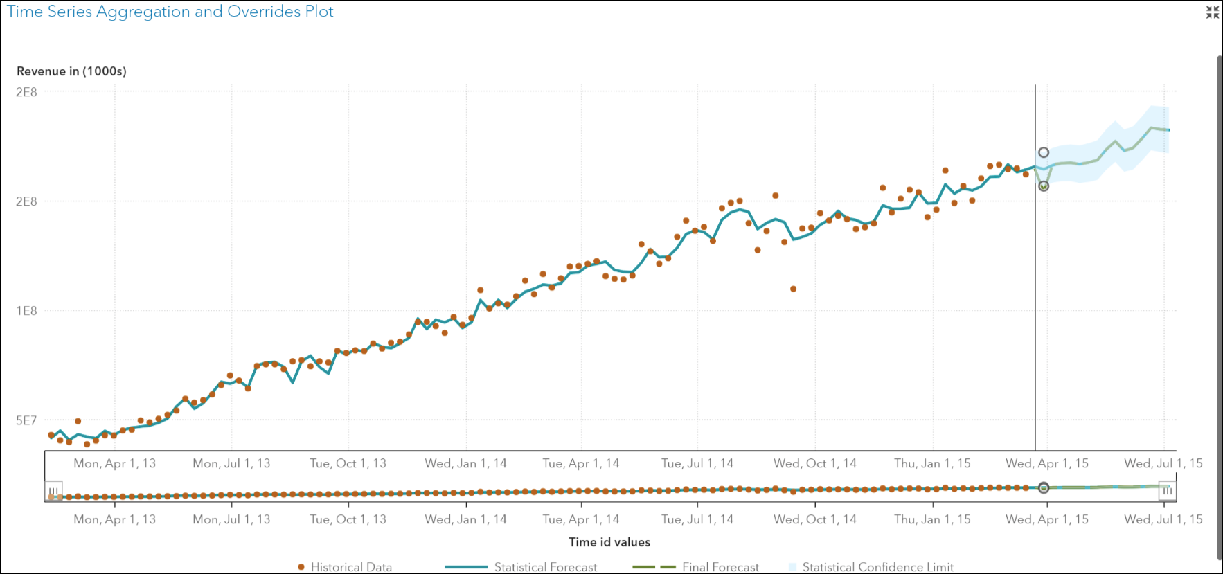
2) a Plot of the Time Series Aggregation and Overrides displaying historical and forecast data, and
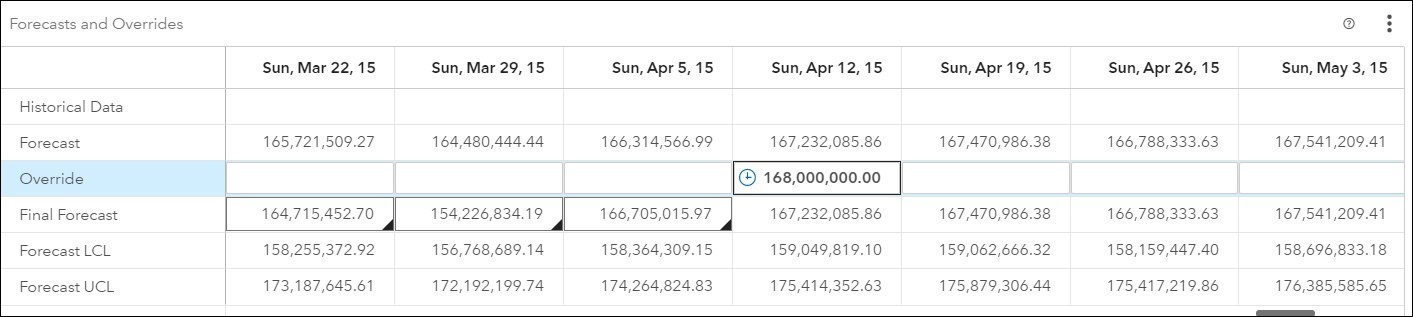
3) a Forecast and Overrides table which can be used to create, edit and submit, override values for a time series based on external factors that are not included in the forecast models
Conclusion
Using SAS Visual Forecasting 8.2 you can effectively model and forecast time series in large scale. The Visual Forecasting Pipeline greatly facilitates the automatic forecasting of large volumes of data, and provides a structured and robust method with efficient and flexible processes.

4 Comments
Hi Patricia,
I picked the UCM model code from pipeline and executed in Code Editor. I used same dataset for both cases. I find Pipeline gives a good forecast but code editor gives a flatline forecast.
Why is this happening?
Rya,
It could be that in the code the default settings for the user interface were not captured. I have two suggestions for you:
1) Take a look at this SAS tutorial video, Using SAS Viya to Create and Fit a User-Specified Mode2) Also, I suggest you open up a Technical Support track for further assistance, they will advise you on the specific settings to add to your code
Regards,
Patricia
Hi Patricia,
Thanks a lot for explaining the entire VF project (forecasting module).
One clarification required is regarding the lead time for the forecasts. I am using forecasting module in project (ESM and ARIMA) and i want to forecast for next 104 weeks.
How can I change it ? Is there a way to put this while creating the project?
Your help will be deeply appreciated.
THanks
Ankush
Ankush,
Hello! Sorry for the delay on replying. I am providing two alternatives because you don’t describe your situation in detail.
This video can be useful for you:
Using SAS Viya to Automatically Model and Forecast Time Series Data https://video.sas.com/detail/video/5361764615001/using-sas-viya-to-automatically-model-and-forecast-time-series-data
Here are the alternatives:
#1
In TSMODEL you can specify all these Predefined Scalar Values
_FORMAT_
time format, which is either implied by the INTERVAL= option or specified in the FORMAT= option in the ID statement
_HORIZON_
the time ID value that is one period beyond _TEND_
_INTERVAL_
time interval, which is specified in the INTERVAL= option in the ID statement
_LEAD_
forecast horizon or lead, which is specified in the LEAD= option in the PROC TSMODEL statement
_LENGTH_
length of the time series that is associated with the current BY group
_SERIES_
series index or BY-group counter. When PROC TSMODEL runs in a parallel processing environment, the index value is relative to the machine that processes the series or BY group. Therefore, values of _SERIES_ might not be unique and could also vary for multiple executions of the procedure.
_SEASONALITY_
length of the seasonal cycle, which is specified in the SEASONALITY= option in the PROC TSMODEL statement or implied by the INTERVAL= option in the ID statement
_TEND_
the last time ID value over all the BY groups. _TEND_ is independent of the value of the TRIMID= option in the ID statement, but the value of _TEND_ is the same as the ending value of the output time ID variable span if you specify TRIMID=NONE.
_TSTART_
the first time ID value over all the BY groups. _TSTART_ is independent of the value of the TRIMID= option in the ID statement, but the value of _TSTART_ is the same as the starting value of the output time ID variable span if you specify TRIMID=NONE.
#2
You could use the atsm package calling it thru proc tsmodel
proc tsmodel data = mylib.pricedata
outobj = (outFor = mylib.outFor(replace = YES)
outEst = mylib.outEst(replace = YES)
outStat = mylib.outStat(replace = YES)
modInfo = mylib.modInfo(replace = YES)
outSel = mylib.outSel(replace = YES));
by regionname productline productname;
id date interval=month;
var sale /acc = sum;
var price/acc = avg;
/*IMPORTANT: use ATSM package */
require atsm;
You will need to declare ATSM Objects, and then use something similar to this:
submit;
/*declare ATSM objects */
declare object dataFrame(TSDF);
declare object diagnose(DIAGNOSE);
declare object diagSpec(DIAGSPEC);
declare object forecast(FORENG);
declare object outFor(OUTFOR);
declare object outEst(OUTEST);
declare object outStat(OUTSTAT);
declare object modInfo(OUTMODELINFO);
declare object outSel(OUTSELECT);
/*setup dependent and independent variables for the data frame*/
rc= dataFrame.initialize();
rc= dataFrame.addY(sale);
rc= dataFrame.addX(price, 'required', 'no', 'extend', 'stochastic');
/*setup time series diagnose specifications */
rc= diagSpec.open();
rc= diagSpec.setArimax('identify', 'both');
rc= diagSpec.setEsm('method', 'best');
rc= diagSpec.setTransform('transform', 'auto');
rc= diagSpec.close();
/*diagnose time series to generate candidate model list*/
rc= diagnose.initialize(dataFrame);
rc= diagnose.setSpec(diagSpec);rc= diagnose.run();
/*run model selection and forecast */
rc= forecast.initialize(diagnose);
rc = forecast.setOption('criterion','rmse');
rc = forecast.setOption('lead', 12, 'holdoutpct', 0.1);
rc= forecast.run();
/*collect forecast results */
rc= outFor.collect(forecast);
rc= outEst.collect(forecast);
rc= outStat.collect(forecast);
rc= modInfo.Collect(forecast);
rc= outSel.Collect(forecast);
endsubmit;
run;
Finally, the SAS documentation is very useful, here is a link for Visual Forecasting
https://support.sas.com/software/products/visual-forecasting/index.html#s1=2
Best,
Patricia