
To make accurate predictions, it is necessary that the sample data you use for model development is compatible with the target population. The distribution of each input used in the model should be similar in the sample and the target population. In your model you should include only those variables which will be available at the time of prediction.
- Compatibility is assured if the data you use for developing the predictive model is from a representative sample drawn from the target population.
- But if you developed your model from a sample that is not drawn from the target population, you need to check if the input ranges are the same in the sample and the target population. If you do not have information on the inputs in the target population, you must at least compare the distribution of some general characteristics such as age, income, education, ethnicity, etc. in the population and the sample.
- When you use time dependent inputs such as customer transactions in your model, and if you use the model to make predictions for a future period, you should make sure the variables included in the model will be available at the time of prediction. Because there may be a lag between the time a transaction takes place and the time at which it is recorded in the data. This lag is called the operational lag. To account for the operational lag, you must define the performance window and prediction window carefully as illustrated below.
An real-world example
For example a bank wants to develop an early warning system to identify customers who are most likely to close their investment accounts in the next three months. The event of a customer closing her account can be called “attrition”. Suppose the bank wants to develop an attrition model to be used as an early warning system for identifying customers who are likely to attrit (close accounts) in the immediate future period such as the next three months. In an attrition model, the target is attrition. The event that a customer closes her account is called attrition. In a modeling data set attrition is a binary variable. The customer record in the modeling data set for developing an attrition model consists of three types of variables (fields):
- Variables indicating the customer’s past transactions (such as deposits, withdrawals, purchase of equities, etc.) by month for several months
- Customer characteristics (demographic and socio-economic) such as age, income, lifestyle, etc.
- Target variable indicating whether a customer attrited during a pre-specified interval
Assume that the model was developed during December 2006, and that it was used to predict attrition for the period January1, 2007 through March 31, 2007.
Display 1 shows a chronological view of a data record in the data set used for developing the attrition model.
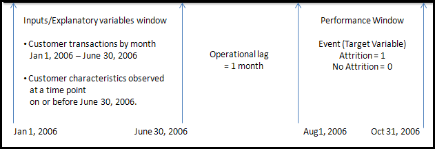
Here are some key input design definitions that are labeled in Display 1:
- inputs/explanatory variables window:
This window refers to the period from which the transaction data is collected. - operational lag:
The model excludes any data for the month of July 2006 to allow for the operational lag that comes into play when the model is used for forecasting in real time. This lag may represent the period between the time at which a customer's transaction takes place and the time at which it is recorded in the data base and becomes available to be used in the model. - performance window:
This is the time interval in which the customers in the sample data set are observed for attrition. If a customer attrited during this interval, then the target variable ATTR takes the value 1; if not, it takes the value 0.
The model should exclude all data from any of the inputs that have been captured during the performance window.
If the model is developed using the data shown in Display 1 and used for predicting, or scoring, attrition probability for the period January 1, 2007 through March 2007, then the inputs window, the operational lag, and the prediction window look like what is shown in Display 2 when the scoring or prediction is done.
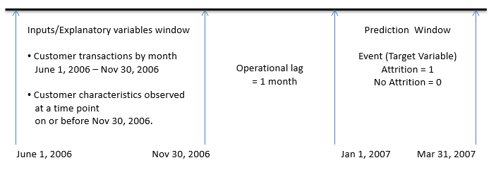
At the time of prediction (say on Dec 31, 2006), all data in the inputs/explanatory variables window is available. In this hypothetical example, however, the inputs are not available for the month of December 2006 because of the time lag in collecting the input data. In addition, no data is available for the prediction window, since it resides in the future (see Display 2).
Since model developed using the data represented by Display 1, it takes into account the operational lag and hence it is consistent with the data available for prediction as shown in Display 2.
For a detailed discussion of the attrition model, see Chapter 7 of my book, Predictive Model with SAS Enterprise Miner™: Practical Solutions for Business Applications, Third Edition. Cary, NC: SAS Institute Inc.
⇒ When you develop a forecasting model using current and recent period data and use the model to make forecasts for the future, it is impossible to check the input ranges in the sample with those forecast period. But we can check the coefficient stability, do cross validation and also construct confidence intervals for the forecasts.