The State Fair in North Carolina is just a few miles from SAS headquarters, and therefore it's virtually impossible for it to slip by without me noticing it. There are two aspects of the fair that usually get lots of news coverage - what's the latest fair-food, and did we set any attendance records? There's not a lot of data about the food available (although I did create this fun graph a few years ago), but thankfully attendance numbers are published on the NC State Fair website daily!
Before we get started, here's an awesome photo my friend John took at this year's State Fair (be sure and click to see the full-size image, so you can take in all the detail!)

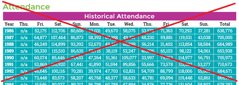
Now, let's analyze that attendance data ... Here's a screen-capture showing the top of the attendance table from the official webpage (click it to see the full table):
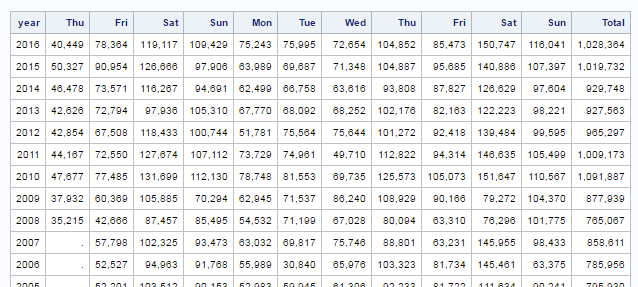
I decided to start my analysis by making a similar table, but with a few enhancements. First, I got rid of the colors, used a '.' rather than 'n/a', and sorted the table with the most recent years at the top. I think all these things make it easier to read.
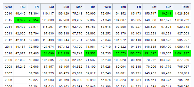
Next, I used some tricky coding techniques to mark the highest attendance for each day in bright green. This involved using user-defined formats with color names, in combination with a somewhat obscure style option in Proc Print. I think this adds important information to the table, and makes it more of an analytic tool rather than just a table. Wow - looks like 2010 had several record-setting days!
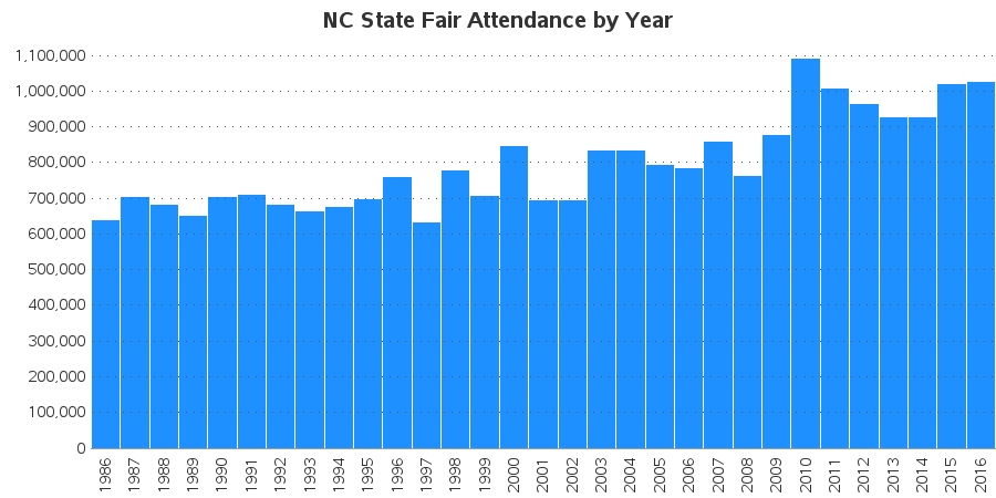
Now that we know which days had the record attendance, let's find out which year had the highest total. And what better way to show that than a simple bar chart! Looks like 2010 was the record setter.
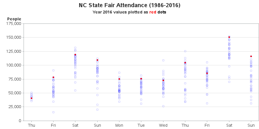
Now, how about some more detailed plots that allow us to visualize all the individual values in the table? Here's a simple plot of the data by day, with the latest (2016) markers in bright red. Note that the other markers are transparent blue, so you can see where multiple markers 'stack up' on top of each other (multiple/overlapping markers become darker, as the transparent colors combine).
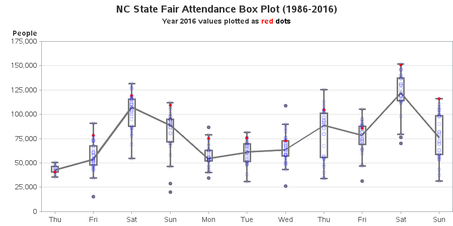
I like that plot, but I'm sure the analysts and statisticians are already salivating for a box plot. I know it's not traditional to show all the markers when using a box plot, but I like to be able to see the spread of the actual data, so I like to include them.
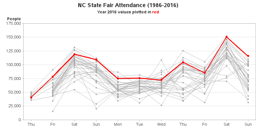
But even the box plot didn't seem to show all the secrets that I knew were hidden in this data. Therefore I created another plot showing each year of data as a separate line - and with this graph, you can see an oddity in the data for the second Thursday (some of the values were high, and some of them were much lower).
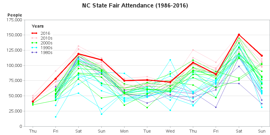
And finally, I decided to color the lines by decade. It's not a beautiful graph (some would even disparagingly call it a spaghetti graph), but in this particular situation I think it provides some important insight that the other graphs did not!
With this graph, I was able to determine that the Thursdays with the lower attendance were from the 1980s and 1990s. And then I remembered that in more recent years there has been a big canned food drive on Thursdays where if you bring 5 cans of food to donate to the Food Bank of Central and Eastern North Carolina, you get into the fair for free. According to the fair website, since 1993, more than 4.4 million pounds of food have been donated by fairgoers. This transformed the traditionally lower-attendance Thursday into one of the higher-attendance days.
Although some portions of NC are still recovering from the flooding caused by Hurricane Matthew, we had nice weather during the fair week this year. This probably helped produce the good attendance numbers. I wonder if it would be possible to correlate fair attendance to weather data? Hmm ... maybe a topic for a future bog!
Another factor which might have helped lure in people this year was the awesome new attraction called the Flyer Sky Ride. It's a chair lift that carries passengers above the fairgrounds, from one end to the other. Here's a link to a cool video my friend David made from this ride.

I hope you had fun exploring & analyzing this data with me, and hopefully you have learned some tricks and techniques to use on your own data!

3 Comments
I have enhanced the interactive graphs so you can now click the plot markers, and see what the weather was like on that particular day! :)
Ksharp - I've run your code, and providing a link to the output, so people who don't have access to run SAS can see what you're suggesting:
http://blogs.sas.com/content/sastraining/wp-content/blogs.dir/24/files/2016/10/SGPanel_nc_statefair_attendance.png
Robert,
It would be look better if you are using Medal Graph.
data have;

infile datalines expandtabs dlm=' ';

input ( Year Thu Fri Sat Sun Mon Tue Wed Thu Fri Sat Sun Total) (: ?? comma32.);

array x{*} Thu--Total;

do i=1 to dim(x);

 x{i}=x{i}/1000;

end;

drop i;

datalines;

1986

n/a

52,175

112,706

80,606

53,031

49,670

58,075

53,576

71,363

70,293

37,281

638,776

1987

n/a

64,877

107,464

86,873

58,392

67,388

49,331

48,230

59,881

119,531

43,038

705,005

1988

n/a

46,249

114,899

93,392

52,670

49,437

68,288

56,214

31,402

113,854

58,584

684,989

1989

n/a

50,330

115,510

86,635

53,715

38,119

52,247

40,096

65,103

98,122

54,061

653,938

1990

n/a

60,074

85,446

71,633

47,264

51,361

109,077

33,997

75,353

114,977

56,791

705,973

1991

n/a

53,869

110,920

67,441

41,890

51,594

89,856

55,666

73,578

112,582

53,277

710,673

1992

n/a

46,646

100,116

70,281

39,974

47,703

62,831

54,709

88,799

118,006

55,606

684,671

1993

n/a

73,448

83,573

58,207

45,768

48,377

58,633

45,781

69,094

119,448

62,861

665,190

1994

n/a

15,546

80,027

89,212

86,798

60,788

47,894

34,876

72,736

131,604

58,802

678,283

1995

n/a

42,479

69,279

89,237

43,358

56,257

58,686

93,179

47,796

130,092

68,940

699,303

1996

n/a

34,455

110,574

89,309

54,391

63,995

43,012

86,285

74,508

131,287

71,613

759,429

1997

n/a

44,106

54,500

28,736

56,008

65,099

82,675

57,399

77,299

136,939

31,379

634,140

1998

n/a

57,948

110,087

94,660

53,131

61,238

55,598

79,440

72,417

122,276

72,561

779,356

1999

n/a

49,812

104,352

19,762

55,650

57,779

26,276

89,598

87,812

136,832

79,574

707,447

2000

n/a

53,331

107,971

94,959

69,580

60,275

58,343

96,904

86,075

137,513

81,773

846,724

2001

n/a

47,940

77,747

46,540

51,921

54,116

57,330

84,975

84,538

113,450

76,620

695,177

2002

n/a

54,036

86,533

80,685

34,563

53,226

73,763

67,634

46,876

118,905

80,756

696,977

2003

n/a

61,364

115,016

97,655

54,579

65,923

64,152

96,614

78,855

129,589

70,208

833,955

2004

n/a

61,289

118,640

95,043

60,296

61,288

57,718

91,556

88,822

119,461

82,206

836,319

2005

n/a

52,201

103,512

90,153

52,983

59,945

61,306

92,233

81,722

111,634

90,241

795,930

2006

n/a

52,527

94,963

91,768

55,989

30,840

65,976

103,323

81,734

145,461

63,375

785,956

2007

n/a

57,798

102,325

93,473

63,032

69,817

75,746

88,801

63,231

145,955

98,433

858,611

2008

35,215

42,666

87,457

85,495

54,532

71,199

67,028

80,094

63,310

76,296

101,775

765,067

2009

37,932

60,369

105,885

70,294

62,945

71,537

86,240

108,929

90,166

79,272

104,370

877,939

2010

47,677

77,485

131,699

112,130

78,748

81,553

69,735

125,573

105,073

151,647

110,567

1,091,887

2011

44,167

72,550

127,674

107,112

73,729

74,961

49,710

112,822

94,314

146,635

105,499

1,009,173

2012

42,854

67,508

118,433

100,744

51,781

75,564

75,644

101,272

92,418

139,484

99,595

965,297

2013

42,626

72,794

97,936

105,310

67,770

68,092

68,252

102,176

82,163

122,223

98,221

927,563

2014	46,478	73,571	116,267	94,691	62,499	66,758	63,616	93,808	87,827	126,629	97,604	929,748

2015	50,327	90,954	126,666	97,906	63,989	69,687	71,348	104,887	95,685	140,886	107,397	1,019,732

2016	40,449	78,364	119,117	109,429	75,243	75,995	72,654	104,852	85,473	150,747	116,041	1,028,364

;

run;

proc transpose data=have out=want;

by year;

run;

ods graphics/width=2000 height=800;

proc sgpanel data=want noautolegend nocycleattrs ;

  panelby _name_ / uniscale=row layout=columnlattice spacing=2 onepanel sort=data novarname;

  dot year / response=col1 group=_name_ nostatlabel

                markerattrs=(symbol=circlefilled size=10);

  rowaxis discreteorder=data display=(nolabel) fitpolicy=none;

  colaxis integer display=(nolabel);

  run;