Do you have fun being a computer geek, and programmatically creating holiday images? If so, then this blog's for you!
In this example, I demonstrate how to take simple x/y coordinates, and create map polygons shaped like holiday images, that can be plotted using SAS/Graph's Proc GMap. Once you learn the basic technique, you can easily re-use this code to create your own images. :)
First, we need some x/y coordinates. I did a few Google searches and found several nice Halloween examples at math-aids.com. I chose the bat, and copy-n-pasted the x/y coordinates into the datalines section of my SAS job. Below is some partial code (you can click here to see the full code) that reads the x/y coordinates into a dataset that can be plotted as a geographical map.
data bat_data; id='bat'; input x y; datalines; 7 6 8 5 9.5 4 11 3.5 13 3 (several data lines not shown) 0 2.5 1 3 3 4 5 5 ; run; |
You can plot the x/y coordinates on a scatter plot, to see what they look like:
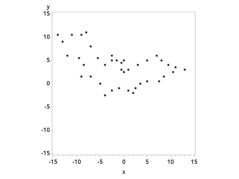
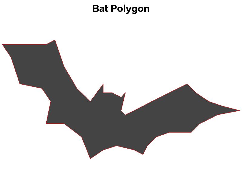
But what we really want is a polygon, filled with a color. You can plot the data as a polygon using Proc GMap, and the polygon named 'bat' will be treated just like a state in the US map:
title "Bat Polygon"; proc gmap data=bat_data map=bat_data; id id; choro id / nolegend coutline=red; run; |
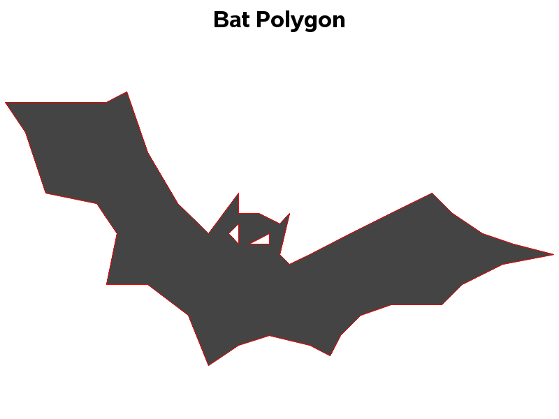
That's pretty good ... but the bat on math-aids.com had eyes. We can create the eyes by making a hole in the map polygon. All you need to do is insert a 'missing' value in the coordinates, and then all the coordinates after that are used to create a hole in the polygon. The following data adds two holes to the bat polygon to create two triangle-shaped eyes:
data bat_data; id='bat'; input x y; datalines; 7 6 8 5 9.5 4 11 3.5 13 3 (several data lines not shown) 0 2.5 1 3 3 4 5 5 . . -3 4 -2.5 4.5 -2.5 3.5 . . -2 3.5 -1 4 -1 3.5 ; run; |
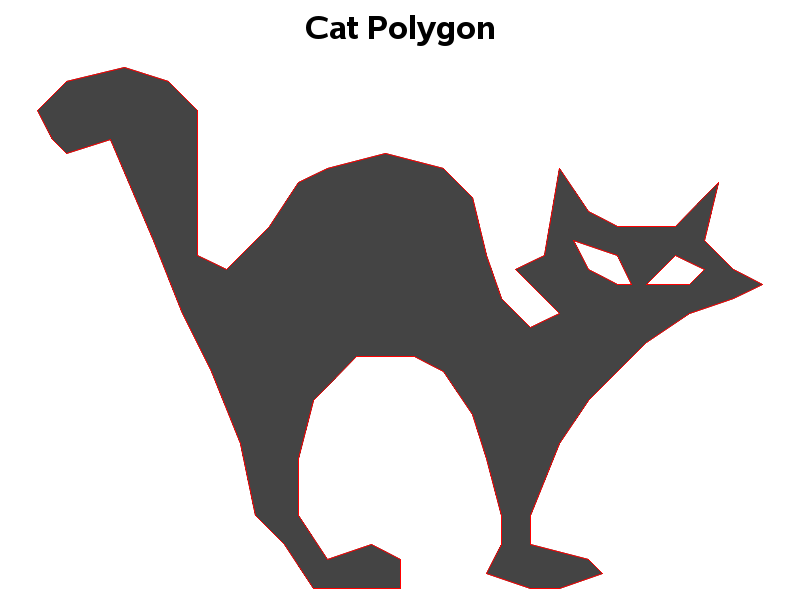
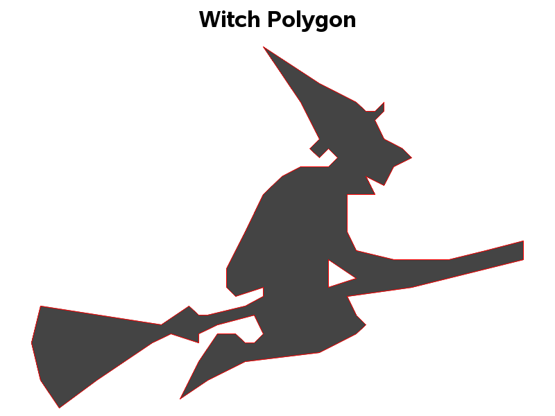
My full code also creates a cat and a witch. If you're teaching someone how to use SAS, you might want to give them the data, and have them try to figure out what the x/y points represent. You could let them try to analyze the data using any proc they want, and then later give them the hint that they might want to try Proc GMap.

4 Comments
Pingback: How to scare up a few good graphs for Halloween - SAS Learning Post
Yes, very fun :-)
In same kind of "business" I made the Homer Simpson plot:
data homer_simpson;
pi=4*atan(1);
do t= 0 to 39*pi by pi/256;
stykke=(t<=3 *pi) *1
+(3 *pi<=t<=7 *pi)*2
+(7 *pi<=t<=11 *pi) *3
+(11 *pi<=t<=15 *pi) *4
+(15 *pi<=t<=19 *pi) *5
+(19 *pi<=t<=23 *pi)*6
+(23 *pi<=t<=27 *pi) *7
+(27 *pi<=t<=31 *pi)*8
+(31 *pi<=t<=35 *pi)*9
+(35 *pi<=t<=39 *pi) *10;
x = ( (-(11/8 )*sin(17/11-8 *t)
-(3/4 )*sin(11/7-6 *t)
-(9/10 )*sin(17/11-5 *t)
+(349/9 )*sin(t+11/7)
+(17/12 )*sin(2 *t+8/5)
+(288/41 )*sin(3 *t+8/5)
+(69/10 )*sin(4 *t+8/5)
+(8/5 )*sin(7 *t+13/8)
+(4/7 )*sin(9 *t+28/17)
+(4/7 )*sin(10 *t+19/11)+1051/8) *(35 *pi<=t<=39 *pi)
+((-3/4 )*sin(11/7-5 *t)
-(54 )*sin(11/7-t)
+(237/8 )*sin(2 *t+11/7)
+(52/11 )*sin(3 *t+33/7)
+(38/9 )*sin(4 *t+11/7)+249/2) *(31 *pi<=t<=35 *pi)
+(-(16/9 )*sin(14/9-5 *t)
-(5/2 )*sin(14/9-3 *t)
+(781/8 )*sin(t+33/7)
+(291/11 )*sin(2 *t+11/7)
+(23/7 )*sin(4 *t+11/7)
+(18/19 )*sin(6 *t+11/7)
+(2/5 )*sin(7 *t+61/13)
+(24/23 )*sin(8 *t+14/9)
+(1/27 )*sin(9 *t+5/11)
+(4/11 )*sin(10 *t+11/7)
+(1/75 )*sin(11 *t+5/8)+1411/7) *(27 *pi<=t<=31 *pi)
+(-(7/11 )*sin(13/10-13 *t)
+(3003/16 )*sin(t+33/7)
+(612/5 )*sin(2 *t+11/7)
+(542/11 )*sin(3 *t+47/10)
+(137/7 )*sin(4 *t+51/11)
+(53/7 )*sin(5 *t+17/11)
+(23/12 )*sin(6 *t+41/9)
+(94/11 )*sin(7 *t+51/11)
+(81/11 )*sin(8 *t+41/9)
+(53/12 )*sin(9 *t+23/5)
+(73/21 )*sin(10 *t+13/9)
+(15/7 )*sin(11 *t+6/5)
+(37/7 )*sin(12 *t+7/5)
+(5/9 )*sin(14 *t+27/7)
+(36/7 )*sin(15 *t+9/2)
+(68/23 )*sin(16 *t+48/11)
+(14/9 )*sin(17 *t+32/7)+1999/9) *(23 *pi<=t<=27 *pi)
+((1692/19 )*sin(t+29/19)
+(522/5 )*sin(2 *t+16/11)
+(767/12 )*sin(3 *t+59/13)
+(256/11 )*sin(4 *t+31/7)
+(101/5 )*sin(5 *t+48/11)
+(163/8 )*sin(6 *t+43/10)
+(74/11 )*sin(7 *t+49/12)
+(35/4 )*sin(8 *t+41/10)
+(22/15 )*sin(9 *t+29/14)
+(43/10 )*sin(10 *t+4)
+(16/7 )*sin(11 *t+6/5)
+(11/21 )*sin(12 *t+55/14)
+(3/4 )*sin(13 *t+37/10)
+(13/10 )*sin(14 *t+27/7)+2383/6) *(19 *pi<=t<=23 *pi)
+(-(1/9 )*sin(7/5-10 *t)
-(2/9 )*sin(11/9-6 *t)
+(20/11 )*sin(t+16/15)
+(7/13 )*sin(2 *t+15/4)
+(56/13 )*sin(3 *t+25/9)
+(1/6 )*sin(4 *t+56/15)
+(5/16 )*sin(5 *t+19/8)
+(2/5 )*sin(7 *t+5/16)
+(5/12 )*sin(8 *t+17/5)
+(1/4 )*sin(9 *t+3)
+(1181/4) *(15 *pi<=t<=19 *pi)
+(-(1/6 )*sin(8/11-5 *t)
+(5/8 )*sin(t+6/5)
+(13/5 )*sin(2 *t+45/14)
+(10/3 )*sin(3 *t+7/2)
+(13/10 )*sin(4 *t+24/25)
+(1/6 )*sin(6 *t+9/5)
+(1/4 )*sin(7 *t+37/13)
+(1/8 )*sin(8 *t+13/4)
+(1/9 )*sin(9 *t+7/9)
+(2/9 )*sin(10 *t+63/25)
+(1/10 )*sin(11 *t+1/9)+4137/8) *(11 *pi<=t<=15 *pi)
+(-(17/13 )*sin(6/5-12 *t)
-(15/7 )*sin(25/26-11 *t)
-(13/7 )*sin(3/14-10 *t)
-(25/7 )*sin(9/13-6 *t)
-(329/3 )*sin(8/17-t)
+(871/8 )*sin(2 *t+2)
+(513/14 )*sin(3 *t+5/4)
+(110/9 )*sin(4 *t+3/8)
+(43/8 )*sin(5 *t+1/5)
+(43/13 )*sin(7 *t+42/11)
+(49/16 )*sin(8 *t+11/13)
+(11/5 )*sin(9 *t+2/7)
+(5/7 )*sin(13 *t+42/13)+1729/4) *(7 *pi<=t<=11 *pi)
+((427/5 )*sin(t+91/45)
+(3/11 )*sin(2 *t+7/2)+5656/11) *(3 *pi<=t<=7 *pi)
+(-(10/9 )*sin(7/10-4 *t)
-(7/13 )*sin(5/6-3 *t)
-(732/7 )*sin(4/7-t)
+(63/31 )*sin(2 *t+1/47)
+(27/16 )*sin(5 *t+11/4)+3700/11) *(t<=3 *pi) ) );
y = ( (-(4/11 )*sin(7/5-10 *t)
-(11/16 )*sin(14/13-7 *t)
-(481/11 )*sin(17/11-4 *t)
-(78/7 )*sin(26/17-3 *t)
+(219/11 )*sin(t+11/7)
+(15/7 )*sin(2 *t+18/11)
+(69/11 )*sin(5 *t+11/7)
+(31/12 )*sin(6 *t+47/10)
+(5/8 )*sin(8 *t+19/12)
+(10/9 )*sin(9 *t+17/11)+5365/11) *(35 *pi<=t<=39 *pi)
+(-(75/13 )*sin(14/9-4 *t)
-(132/5 )*sin(11/7-2 *t)
-(83 )*sin(11/7-t)
+(1/7 )*sin(3 *t+47/10)
+(1/8 )*sin(5 *t+14/11)+18332/21) *(31 *pi<=t<=35 *pi)
+((191/3 )*sin(t+33/7)
+(364/9 )*sin(2 *t+33/7)
+(43/22 )*sin(3 *t+14/3)
+(158/21 )*sin(4 *t+33/7)
+(1/4 )*sin(5 *t+74/17)
+(121/30 )*sin(6 *t+47/10)
+(1/9 )*sin(7 *t+17/6)
+(25/11 )*sin(8 *t+61/13)
+(1/6 )*sin(9 *t+40/9)
+(7/6 )*sin(10 *t+47/10)
+(1/14 )*sin(11 *t+55/28)+7435/8) *(27 *pi<=t<=31 *pi)
+(-(4/7 )*sin(14/9-13 *t)
+(2839/8 )*sin(t+47/10)
+(893/6 )*sin(2 *t+61/13)
+(526/11 )*sin(3 *t+8/5)
+(802/15 )*sin(4 *t+47/10)
+(181/36 )*sin(5 *t+13/3)
+(2089/87 )*sin(6 *t+14/3)
+(29/8 )*sin(7 *t+69/16)
+(125/12 )*sin(8 *t+47/10)
+(4/5 )*sin(9 *t+53/12)
+(93/47 )*sin(10 *t+61/13)
+(3/10 )*sin(11 *t+9/7)
+(13/5 )*sin(12 *t+14/3)
+(41/21 )*sin(14 *t+22/5)
+(4/5 )*sin(15 *t+22/5)
+(14/5 )*sin(16 *t+50/11)
+(17/7 )*sin(17 *t+40/9)+4180/7) *(23 *pi<=t<=27 *pi)
+(-(7/4 )*sin(8/11-14 *t)
-(37/13 )*sin(3/2-12 *t)
+(2345/11 )*sin(t+32/21)
+(632/23 )*sin(2 *t+14/3)
+(29/6 )*sin(3 *t+31/21)
+(245/11 )*sin(4 *t+5/4)
+(193/16 )*sin(5 *t+7/5)
+(19/2 )*sin(6 *t+32/7)
+(19/5 )*sin(7 *t+17/9)
+(334/23 )*sin(8 *t+35/8)
+(11/3 )*sin(9 *t+21/11)
+(106/15 )*sin(10 *t+22/5)
+(52/15 )*sin(11 *t+19/12)
+(7/2 )*sin(13 *t+16/13)+12506/41) *(19 *pi<=t<=23 *pi)
+(-(3/7 )*sin(1/10-9 *t)
-(1/8 )*sin(5/14-5 *t)
-(9/8 )*sin(26/17-2 *t)
+(18/7 )*sin(t+14/11)
+(249/50 )*sin(3 *t+37/8)
+(3/13 )*sin(4 *t+19/9)
+(2/5 )*sin(6 *t+65/16)
+(9/17 )*sin(7 *t+1/4)
+(5/16 )*sin(8 *t+44/13)
+(2/9 )*sin(10 *t+29/10)+6689/12) *(15 *pi<=t<=19 *pi)
+(-(1/27 )*sin(1-11 *t)
-(1/6 )*sin(4/11-10 *t)
-(1/5 )*sin(2/11-9 *t)
-(7/20 )*sin(1/2-5 *t)
-(51/14 )*sin(29/28-3 *t)
+(23/7 )*sin(t+18/5)
+(25/9 )*sin(2 *t+53/12)
+(3/2 )*sin(4 *t+41/15)
+(1/5 )*sin(6 *t+36/11)
+(1/12 )*sin(7 *t+14/3)
+(3/10 )*sin(8 *t+19/9)+3845/7) *(11 *pi<=t<=15 *pi)
+(-(8/7 )*sin(1/3-13 *t)
-(9/13 )*sin(4/5-11 *t)
-(32/19 )*sin(17/12-9 *t)
-(11/6 )*sin(9/13-8 *t)
-(169/15 )*sin(8/17-3 *t)
+(917/8 )*sin(t+55/12)
+(669/10 )*sin(2 *t+4/13)
+(122/11 )*sin(4 *t+49/24)
+(31/9 )*sin(5 *t+1/8)
+(25/9 )*sin(6 *t+6/7)
+(43/10 )*sin(7 *t+1/21)
+(18/19 )*sin(10 *t+9/13)
+(2/9 )*sin(12 *t+31/15)+1309/5) *(7 *pi<=t<=11 *pi)
+(-(267/38 )*sin(3/10-2 *t)
+(625/8 )*sin(t+62/17)+8083/14) *(3 *pi<=t<=7 *pi)
+( (1370/13 )*sin(t+25/6)
+(41/21 )*sin(2 *t+205/51)
+(11/16 )*sin(3 *t+8/13)
+(9/13 )*sin(4 *t+26/9)
+(6/5 )*sin(5 *t+11/14)+2251/4) *(t<=3 *pi) );
output;
end;
drop pi;
*coefficients are calculated in Wolfram Alpha.;
run;
symbol;
%macro symbols;
%do i=1 %to 12;
symbol&i. i=join v=none color=yellow w=2;
%end;
%mend;
%symbols
proc gplot ;
plot y*x=stykke/noaxis nolegend noframe;
run;
Wow - someone must be quite a dedicated Homer Simpson fan to have worked out all that code! I tried running it, and it does indeed produce a very nice drawing!
What fun! Great idea and thanks for the images. If you have SAS 9.4m1, you can also create these images by using the new POLYGON statement in PROC SGPLOT:
proc sgplot data=bat_data;
polygon x=x y=y id=id / outline lineattrs=(color=red)
fill fillattrs=(color=gray44);
xaxis display=none;
yaxis display=none;
run;