For Climate Month I thought I’d research something on the positive side of the equation. My last two climate posts were a bit gloomy, as they focused on greenhouse gasses and ocean acidification. Instead we’re going to tackle a product adoption issue related to the climate: When might the United States reach 50% market saturation for residential solar power?
New Product Marketing: The Bass Diffusion Model
The technique I’m going to employ to answer this question is the Bass Model. Named for it’s creator, professor Frank Bass, then at Purdue University, it’s been a mainstay of new product forecasting for consumer goods since it was first published in 1969. The basic premise of the model is that new product adopters can be classified as innovators or as imitators, and that the overall adoption rate depends on their degree of interaction with the new product.
The generalized formula(s) for the Bass Model are published below at the end of this article. It utilizes just three parameters. N is the market size in units, with p and q representing the adoption rates for innovators and imitators respectively. The innovators simply adopt the new product at some rate depending on the characteristics of the product and their needs. The imitator’s rate of adoption, however, depends on how many innovators have already adopted the new product. While I’ll be using cumulative adoption numbers in order to ascertain market saturation, using incremental adoption quantities gives you the recognizable bell curve of the product lifecycle: Innovators, early adopters, early majority, late majority and laggards.
Parameter estimates
While N, the total market size, is generally relatively easy to obtain a ballpark number for, the adoption rates, p and q, are more difficult. A number of studies over the decades have compiled databases of p and q adoption rate values for a variety of specific products (e.g. air conditioners) and for general product categories (e.g. consumer durable goods). As the basis for this exercise I’m going to use the work of Wharton marketing professor Christophe Van den Bulte – as solid a quantitative starting point as any out there.
Van den Bulte compiled a database of nearly 1,600 p and q innovator and imitator adoption rates for various product and geography combinations, which he eventually reduced to about 200 more generalized parameter sets. For the baseline category of consumer durable goods he gives us a p innovator rate of 0.016 and a q imitator value of 0.41. This is well in line with other p/q database references where the ranges seem to fall between 0.01 and 0.025 for p, and 0.2 and 0.8 for q. He then offers adjustments to this general baseline, of which we will use, for reasons explained below, his adjustments for cell phones: 0.226 and 0.635 respectively. Multiplied together this gives us prospective p and q adoption rates of 0.003 and 0.26 for residential solar panels.
Choosing cell phones as the initial analog is based on the similarity of both products in their requirements for infrastructure – cell towers in one case, and government/utility regulations permitting connections to the network in the other. This approach is reinforced by recent studies of the emerging EV (electric vehicle) market, where p seems to be in the 0.001 to 0.003 range, and q between 0.2 and 0.8 – another market highly dependent on infrastructure.
There are about 87 million detached single-family homes in the United States, which I’ll define as our target market. Of these, only about 80% have suitable rooftop space for a minimal 1.5 KW unit (with 5 to 6 KW being the average installation), and only about 80% of these are located in areas with viable sunlight conditions, giving us an N of about 55 million homes.
Testing some parameters
We have numbers for installed homes to use both as our 2019 starting point and to test the accuracy of the model. In the year 2000 there were 47,000 homes installed with solar panels, which grew to 200,000 in 2010 and 700,000 by 2019. Those 700,000 homes represent about 1% of the total market, and generate around 0.6% of the total electricity produced in the country. Currently the industry is predicting about 1.5 million installations by 2023 – four years from now.
Our first bit of trouble arises when we try to fit our model to the 2000-2019 data, where it concludes that we should have 27 million installed homes today – that’s only off by a factor of 40 from the real number of 700,000.
Slightly more promising is the approach of taking q to zero (more on why, below), where we get a 2019 projection of about 3 million homes – off by only a factor of 4 instead of 40. Additionally reducing p to 0.001, as for some of the EV models, gives us about one million – pretty close – but with no real rationale for reducing that p innovator rate. Lastly, if we drop q to zero, keep p at 0.003, but reduce our N, our market size, to 12 million, we get 700,000.
Chasms and infrastructure
What’s the justification for reducing q to zero? Geoffrey Moore’s “Crossing the Chasm” introduces the concept of a chasm between the innovators/early adopters and the rest of the market - the majority and the laggards. According to Chasm theory, moving from the early adopter to the early majority stage is not just a matter of incremental growth - there is a significant threshold to be crossed - a difference in kind and not just degree. What if we’ve been using the Bass Model too loosely? What if the imitators, the “q’s”, don’t come into play until AFTER we’ve crossed the chasm?
I will describe how this plays out shortly, but I first want to also justify the market size reduction to 12 million. What if in the early stages of an infrastructure-dependent new product you need to restrict your view of the total market to only that portion where the infrastructure has had a chance to develop in order to create accurate forecasts? In the rollout of residential solar panels many states and local/regional utilities had no regulatory, financial or technical provisions in place to accept residential connections to the network. Perhaps it will be many years or decades before we can consider the market to be the entire 55 million eligible homes.
Having already invoked Geoffrey Moore and “Crossing the Chasm” in defense of a zero q value, I’d like to reintroduce W. Brian Arthur and his “The Nature of Technology” from my earlier blog, “Analytics and Innovation,” where professor Arthur segments innovations into four types: phenomenon, devices, combinations, and systems. This last one, systems, is highly infrastructure dependent and might serve as a theoretical basis for limiting the market size N.
It may be that most of our historically computed p and q adoption rates come from product innovations that fall predominantly into the device and combination categories where they are not so dependent on infrastructure, and thus are not well-suited as analogs for system-level innovations, such as cell phones, EVs and solar panels.
Residential solar market saturation
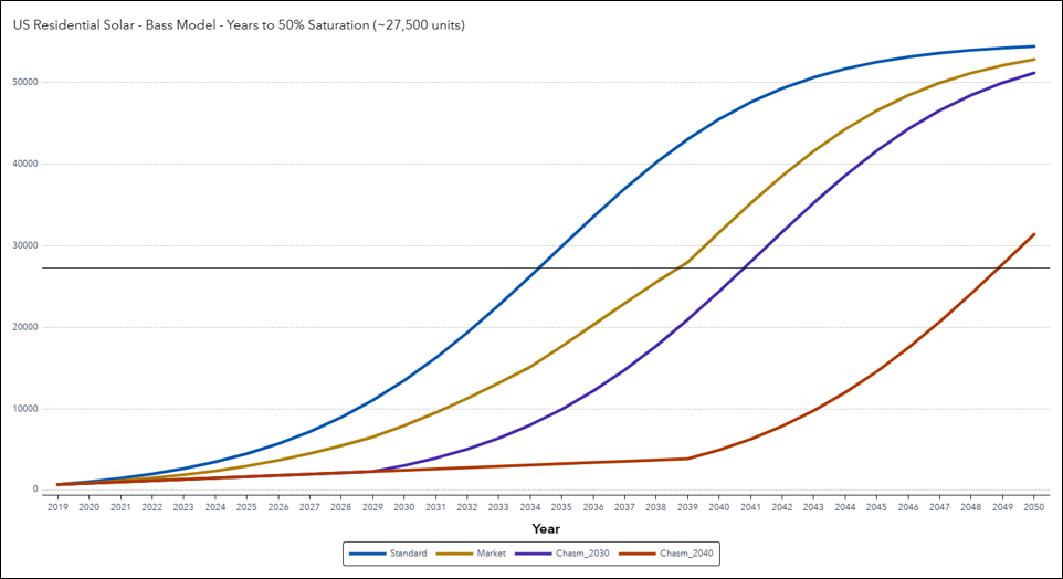
Where does this leave us? The graph shows four scenarios (out of dozens of possible combinations) built upon the chasm and infrastructure approaches described above. The STANDARD scenario (blue) utilizes our baseline p and q adoption rates and fails miserably right out of the starting blocks, where it predicts 2.7 million installations by 2013 when the industry is saying only half that. The Standard model would have us at 50% market saturation by 2035.
The MARKET model (gold) also utilizes the baseline p and q parameters but progressively limits the addressable market size N, starting with 15 million homes in 2020 and increasing by 5 million every five years thereafter. It roughly matches current industry projects for 1.5M to 2.0M installations by 2013, and reaches 50% saturation around 2040.
The two chasm-based models (purple and red) leave the market size N at 55 million but reduce q to zero until 2030 and 2040 respectively, after which the Standard 0.26 value kicks in, with commensurate 50% saturation dates of roughly 2040 and 2050, reflecting a market dynamic where there are only innovators and no imitators until some critical mass is reached or threshold crossed.
Overall the models seem to indicate a range of no earlier than 2040 but almost certainly by 2050. Trying to get more exact than this twenty years out may be a fools game, but if you needed a more precise estimate you’d have to make a definitive choice for modelling approach.
Which approach is best?
We’ve been using the Bass Model for decades as a basis for new product forecasting, and while it seems to work well for homogeneous product categories, it does a less satisfactory job with certain outlier technologies and innovations, such as EVs and solar panels. Incorporating the ideas mentioned above will first require validation using actual historical data.
Is there any evidence for a Chasm effect? It may not be there, or, because we were never looking for it, it might jump out of the data when viewed through the proper lens. Can a case be made for evolving addressable markets? This one seems to be the easier of the two to support, but might only be applicable in a minority of infrastructure-dependent situations, irrelevant to the bulk of the device/combination consumer durable market.
If either or both of these effects bear out, then we will likely find a trade-off between the benefit of a narrower range of p and q rates applicable to a wider set of products, but the additional requirement of needing to estimate when the chasm gets crossed or how the addressable market size evolves, neither of which may emerge in a generalizable form from the historical data. A hybrid model incorporating both effects simultaneously may even be justified, or it may end up being a just another case of overfitting to the training data. In the end, model simplicity but with wider confidence intervals may still turn out to be the better approach.
Learn about the SAS commitment to people and the planetBass Model Formulations:
- Incremental Bass Model: n(t) = [N – N(t-1)] (p + q[N(t-1)/N]) (gives you the product lifecycle bell curve)
- Cumulative Bass Model: N(t) = [N – N(t-1)] (p + q[N(t-1)/N]) + N(t-1) (gives you the saturation S-curve)