Hidden Markov Models
Introduction
Statistical models of hidden Markov modeling (HMM) have become increasingly popular in the last several years. The models are very rich in mathematical structures and can form the theoretical basis of many real applications. In the classical continuous/discrete Markov process, each state corresponds to an observed (physical) event. The hidden Markov modeling focuses on the case where the observation is a probabilistic function of the hidden state. In other words, the hidden Markov model is a doubly embedded stochastic process with an underlying stochastic process hidden (unobservable) and another observable stochastic process producing the sequence of observations.
Elements of an HMM
An HMM is characterized by the following five key elements:
, the number of hidden states. Denote the set of states by
.
- Initial state probability vector (ISPV),
.
- Transition Probability Matrix (TPM),
where
.
, the number of distinct observation symbols per state.
, The probability distribution of observation symbols for each state
.
The set of model parameters is denoted by .
The HMM Procedure/Action set
Given the sequence of observations , a basic problem of interest to be addressed for the HMM in real-world applications is: How do we adjust model parameters
to maximize the probability of observing such a sequence of observations, that is,
? The HMM procedure in SAS Econometrics 8.5 (its corresponding CASL version is the HMM action) was developed to solve the problem, that is, to adjust model parameters to maximize the probability of the observation sequence given a model.
Regime-Switching Autoregression Model
We attempt to fit the observation sequence to the Regime-Switching model when the parameters of the data generating process (DGP) vary over a set of different unobserved states. The Regime-Switching Autoregression (RS-AR) model allows states to switch according to a Markov process and is often applied to lower frequency data (quarterly, yearly, and so on). A typical application of such a model is stock returns. Generally, the RS-AR model can be formulated as follows:
where
: Dependent variables.
: State-dependent intercept/mean.
: Vector of exogenous variables with state-dependent coefficients
.
:
-th AR term in state
.
: i.i.d. normal distribution
.
: order of regression.
Two key methods for parameter estimation include the maximum a posteriori method (MAP) and the maximum likelihood method (ML). Three optimization algorithms supported by the HMM action are the active-set algorithm, the interior-point algorithm, and the stochastic gradient descent algorithm. As the HMM solver iteratively updates and improves model parameters, the choice of initial parameters is crucial in searching for a good local optimizer.
An example: Discovering the Hidden Market States
Each RS-AR model is characterized by the number of states and the order of regression
. Given a fixed pair
, we can use the HMM action set to estimate the model parameters. The sequence of observations used in the numerical experiments is called vwmi and is extracted from the CRSP data. In the example, we tested 48 models with
and
. In order to select a good initial point for the iterative procedure, the multistart mode is enabled. The following CASL script shows how to call the HMM solver and get estimation results for all 48 AR models.
%macro estimateRSAR(myds, inEstDs, kStart, kEnd, pStart, pEnd, method, maxiter, qMultiStart);
   proc cas;
      hiddenMarkovModel.hmm result=r/
         data = {caslib='casuser', name="&myds."},
         id={time='date'},
         outstat={name="&myds.&method.Stat_k&kStart.To&kEnd._p&pStart.To&pEnd.", caslib="casuser", replace=true},
         model={depvars={'returnw'}, method="&method.", nState=&kStart., nStateTo=&kEnd., ylag=&pStart., yLagTo=&pEnd., type = 'AR'},
         optimize = {algorithm='interiorpoint', printLevel=3, printIterFreq=1, maxiter=&maxiter., Multistart = &qMultiStart.},
         score = {outmodel={name = "&myds.&method.Model_k&kStart.To&kEnd._p&pStart.To&pEnd.", caslib="casuser", replace=true}},
         learn = {out={name = "&myds.&method.Learn_k&kStart.To&kEnd._p&pStart.To&pEnd.", caslib="casuser", replace=true}
                  %if %length(&inEstDs.)>0 %then %do; , in={name = "&inEstDs.", caslib="casuser"} %end;},
         labelSwitch={sort="NONE"},
         display = {names = {"Optimization.Algorithm", "ModelInfo", "ParameterMatrices.TPM", "Optimization.FinalParameterEstimates", "Optimization.IterHistory",
                             "FitStatistics", "Optimization.InitialObjectiveFunction", "Optimization.FinalObjectiveFunction"}};
        print r;
   run; quit;
   CAS mysess listhistory;
%mend;

/*use MAP and enable multistart for p = 0 models to obtain initial parameter estimations*/
%estimateRSAR(myds=vwmi, inEstDs=, kStart=2, kEnd=9, pStart=0, pEnd=0, method=MAP, maxiter=128, qMultiStart=1);

/*use ML and disable multistart for p = 0 to 5 models to get final paramter estimations*/
%estimateRSAR(myds=vwmi, inEstDs=vwmiMAPLEARN_K2TO9_P0TO0, kStart=2, kEnd=9, pStart=0, pEnd=5, method=ML, maxiter=128, qMultiStart=0);
For AR models with , the common practice is first to take MAP as the estimation method and enable multistart mode to get an initial parameter estimate. Then we take the output of the MAP method to hot-start the ML method, using output parameter estimates as the initial values and calling the HMM procedure the second time using the ML method. For the other models of
, the HMM solver automatically takes outputs from the corresponding AR (
) model as initial values.
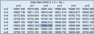
To compare the quality of different statistical models, we could measure the Akaike information criterion (AIC) value, which is basically an estimator of out-of-sample prediction error. Therefore, the minimal AIC value in the following table identifies the best model () among the 48 AR models. Note that the multistart mode of the HMM action takes around 17 hours to get the full AIC table as it currently supports only single-machine mode. Refer to Example 13.1 in the HMM documentation for a more detailed interpretation.
Black-Box optimization solver
The black-box optimization solver has rich applications in hyperparameter tuning whose objective functions are usually nonsmooth, discontinuous, and unpredictably varying in computational expense. The hyperparameters we want to tune might be mixtures of continuous, categorical, and integer parameters. The solveBlackbox action was developed based on an automated parallel derivative-free optimization framework called Autotune. Autotune combines a number of specialized sampling and search methods that are very efficient in tuning complex models like in machine learning. The Autotune framework is illustrated in Fig.2. Autotune has the ability to simultaneously apply multiple instances of global and local search algorithms in parallel, among which a global algorithm is first applied to determine a good starting point to initialize a local algorithm. An extended suite of search methods is driven by the Hybrid Solver Manager that controls concurrent execution of different search methods. One can easily add new search methods to the framework. Overall, search methods can learn from each other, discover new opportunities, and increase the robustness of the system.
The solveBlackbox action based on the Autotune framework takes the Genetic Algorithm (GA) as the global solver and Generating Set Search (GSS) to perform local search in a neighborhood of selected members from the current GA population. It is notable that the solveBlackbox action can handle more than one objective and support both linear and nonlinear constraints. Furthermore, it can work well in either single-machine mode or distributed mode.
Due to the existence of many local optima, the choice of starting points (called initial values) in HMM has a significant impact on the quality of the solution. The usage of multistart mode helps identify a better initial point and hence better local optimum at the expense of time. The black-box optimization solver is a good alternative to the multistart approach due to the following key properties:
- The HMM objective function is a black-box function of the initial values/parameters. Most importantly, we do not need to have an explicit mathematical form of such an objective function. It might be smooth or nonsmooth, continuous or discontinuous, very expensive in function value evaluations, and so on.
- The hyperparameters considered in the black-box optimization solver could be continuous (for example, the initial values), integer (for example, the number of states and the order of regression), as well as categorical (for example, type of methods and algorithms).
- The black-box optimization solver supports parallel function evaluations automatically, which parallelizes multiple HMM procedures starting from different initial points.
Numerical Experiments
We then take initial values as the tuning hyperparameters. Specifically, the set of hyperparameters to be tuned includes three sets of variables: 1) Transition probability matrix of hidden states, where each row sums up to one and all elements should be nonnegative; 2) State-dependent intercepts, which can be any real numbers; 3) Covariance matrix or variance, which should be positive semidefinite or nonnegative.
Three configurations in solveBlackbox are tested for tuning hyperparameters for two data sets (vwmi and jpusstock).
- Blackbox-MAP: Tuning models with
using the MAP estimation method.
- Blackbox-ML: Tuning models with
using the ML estimation method.
- Blackbox-ML-All: Tuning each model (any
,
) using the ML estimation method.
The following example code demonstrates how we use the solveBlackbox action to tune HMM initial values.
%macro TuneHmm(ns, nvars, pStart, maxgeneration, method, maxiter);
proc cas noqueue;
   /*use an Initial function to load data to servers*/
   source casInit;
      loadTable / caslib='casuser', path='vwmi.sashdat', casout='vwmi';
   endsource;

   /*specify blackbox objective function*/
   source caslEval;
      hiddenMarkovModel.hmm result=r /
         data = "vwmi",
         id={time='date'},
         model={depvars={'returnw'}, method="&method.", nState=&ns., ylag=&pStart., type = 'AR'},
         initial={'TPM={' || (String) x1 || ' ' || (String) x2 || ', ' || (String) x3 || ' ' || (String) x4 || '}',
                  'MU={'|| (String) x5 || ', ' || (String) x6 || '}',
                  'SIGMA={' || (String) x7 || ', ' || (String) x8 || '}'}, /*the initial value list is different for different nState*/
         optimize = {algorithm='interiorpoint', printLevel=3, printIterFreq=1, maxiter=&maxiter., Multistart = 0},
         score= {outmodel={name = "&ds.&method.Model_k&ns.p&pStart._" || (String) _bbEvalTag_ || "_&nworkers.", caslib="casuser", replace=true}},
         learn= {out={name = "&ds.&method.Learn_k&ns.p&pStart._" || (String) _bbEvalTag_ || "_&nworkers.", caslib="casuser", promote=true}},
         labelSwitch={sort="NONE"};
      f['obj1'] = r.FitStatistics[1, 2];  /*read log likelihood value from FitStatistics table*/
      send_response(f);
   endsource;

   /* Invoke the solveBlackbox action */
   optimization.solveBlackbox result=blackr/
      decVars = myvars, /*define tuning variables as the initial values of hmm*/
      obj = {{name='obj1', type='max'}},
      maxGen= &maxgeneration., /* by default 10 */
      popSize=15, /* by default 40 */
      maxTime = 3600,
      linCon={name = "lindata", caslib = "casuser"}, /*read coefficients of linear constraints from lindata*/
      func = {init=casInit, eval=caslEval},
      nParallel=30; /* specify the number of parallel sessions*/
run; quit;
%mend;

/* call the tuning process for any k, p */
%TuneHmm(ns = 2, nvars = 8, pStart = 0, maxgeneration = 5, method = MAP, maxiter = 128); /*Blackbox-MAP*/
%TuneHmm(ns = 2, nvars = 8, pStart = 0, maxgeneration = 1, method = ML, maxiter = 128); /*Blackbox-ML and Blackbox-ML-All*/
Tuning RS-AR models with ![p = 0]()
Instead of using multistart for models, we use the solveBlackbox action to tune
models using MAP and ML, denoted Blackbox-MAP and Blackbox-ML, respectively. Then we run the second-stage optimization using ML as the multistart did to obtain the full AIC table.
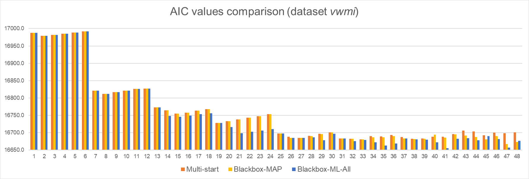
First data set vwmi: For this vwmi data set, we considered values of ranging from 2 to 9, and values of
from 0 to 5. The following histogram shows the comparison of AIC values for Multistart, Blackbox-MAP, and Blackbox-ML. The 48 models are ordered by
and
in ascending order. The model with
and
is indexed by 1, the model with
and
is indexed by 2, and so on.
 The results tell us the black-box optimization solver does help identify a better local optimum among half of the 48 models, especially when the model size is large. Compared with multistart mode, Blackbox-MAP is 76% faster and Blackbox-ML is 91% faster. Overall, Blackbox-MAP performs slightly better than Blackbox-ML in terms of solution quality, while Blackbox-ML is more computationally efficient than Blackbox-MAP.
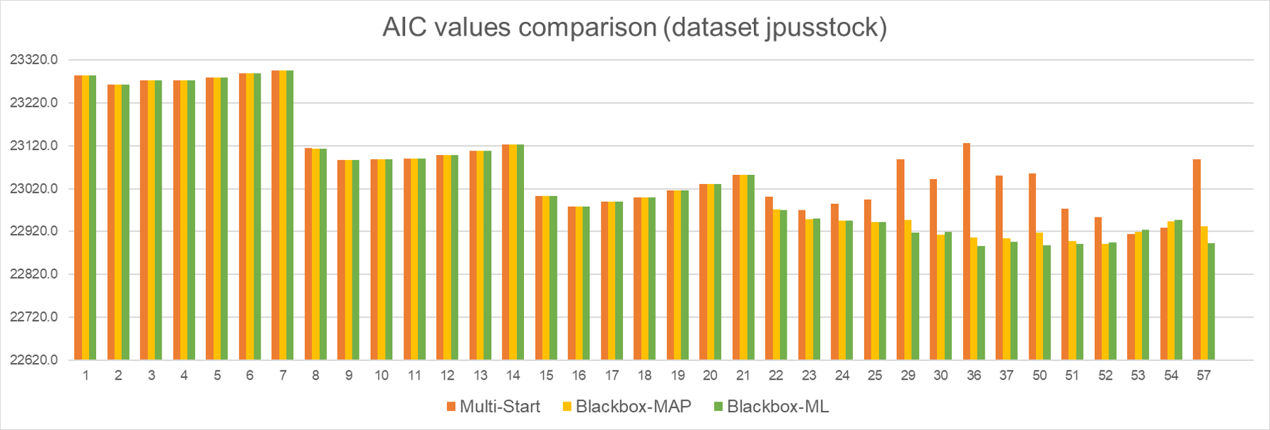
Second data set jpusstock: This data set contains two sets of historical weekly returns and results in RS-AR models of two dependent variables. Considering AR models with and
, some of the resulting AIC values of Multistart, Blackbox-MAP, and Blackbox-ML are presented below. Except for two models (
,
and
), Blackbox-MAP and Blackbox-ML lead to a solution that is at least as good as Multistart, with significant improvements in large models. Furthermore, both tuning configurations are 90% faster than the Multistart method.
Note that among 63 models, the Multistart method is able to help find a reasonable parameter estimation for 39 models, while Blackbox-MAP and Blackbox-ML work for 48 and 50 models, respectively. These results indicate that using the output for from these methods does not necessarily work well in the second-stage optimization. A possible good solution for this case is explored in the next experiments, that is, tuning each model directly using ML.
Tuning RS-AR models with any ![k]() ,
, ![p]()
Due to the ill-posed objective functions of HMM, we observed that the two-stage strategy based on results from Multistart, Blackbox-MAP, and Blackbox-ML sometimes results in unrealistic parameter estimations, especially for models. For instance, the eigenvalues of the covariance matrix in one of the hidden states are very close to zero when
. This motivates us to try to find a good initial point for any model directly. Therefore, we further consider tuning each model directly using ML, denoted Blackbox-ML-All. The resulting AIC values from this strategy are compared with Multistart and Blackbox-MAP for both data sets.
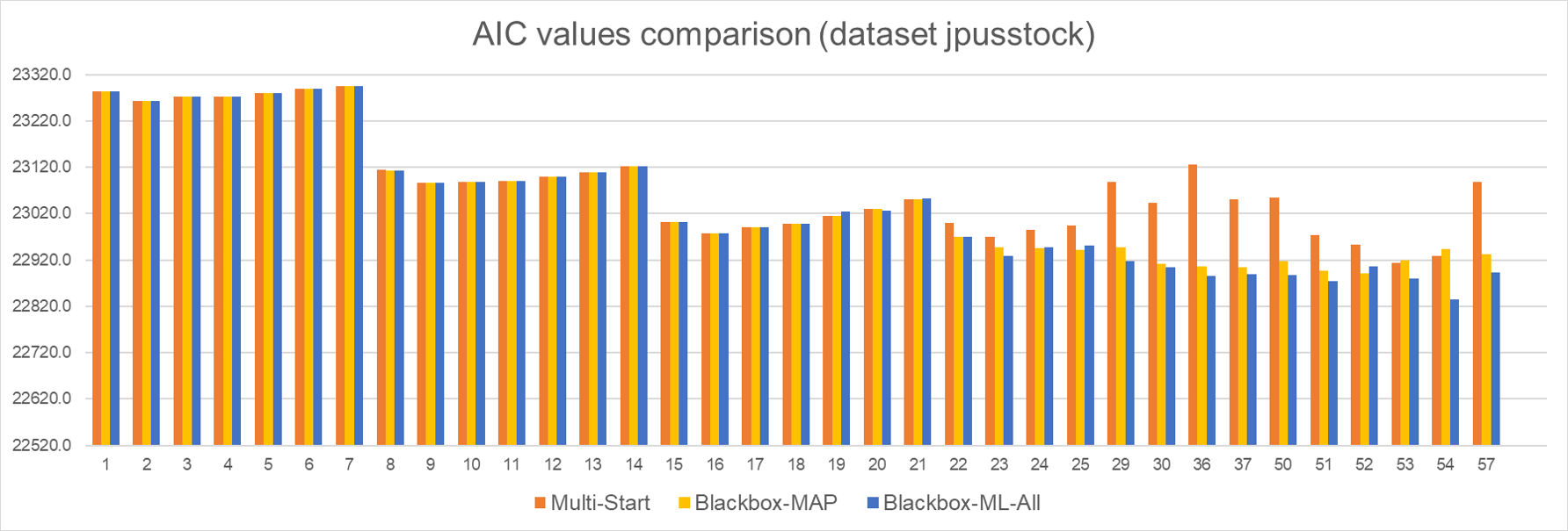
We can see from the above results that Blackbox-ML-All further improves the solution quality for most of the models, though the time of Blackbox-ML-All is around six times slower than Blackbox-ML. Despite Blackbox-ML-All being slower than Blackbox-ML, it provides higher quality solutions and is still 50% faster than Multistart in finding the best model and the corresponding parameter estimation. More importantly, for the second data set, Blackbox-ML-All is able to produce good final parameter estimations for all 63 models. Therefore, we believe that Blackbox-ML-All is a good alternative to Multistart mode whenever Multistart results in bad estimations of parameters.
Summary
The multistart mode supported by the HMM procedure and the HMM action can only run in a single machine, leading to high time cost. The numerical test for the data set jpusstock revealed that multistart is not reliable to find a good estimation of parameters. Given that the solveBlackbox action supports parallel function evaluations and applies to any type of black-box functions and hyperparameters, we frame the solveBlackbox action to tune the initial values for the HMM. Exploring three different black-box tuning configurations, we are able to improve the solutions of the HMM models in terms of both solution quality and computational cost. In conclusion, the black-box optimization solver is a good alternative to identify good initial parameter estimates in the HMMs.
References
[1] Patrick Koch, Oleg Golovidov, Steven Gardner, Brett Wujek, Joshua Griffin, and Yan Xu. 2018. Autotune: A Derivative-free Optimization Framework for Hyperparameter Tuning. In KDD. 443--452.
[2] S. Gardner et al., "Constrained Multi-Objective Optimization for Automated Machine Learning," 2019 IEEE International Conference on Data Science and Advanced Analytics (DSAA), Washington, DC, USA, 2019, pp. 364-373, doi: 10.1109/DSAA.2019.00051.
[3] L. R. Rabiner, "A tutorial on hidden Markov models and selected applications in speech recognition", Proc. IEEE, vol. 77, pp. 257-286, Feb. 1989.
[4] Kim, C.-J., C. R. Nelson, and R. Startz. 1998. Testing for mean reversion in heteroskedastic data based on Gibbs-sampling-augmented randomization. Journal of Empirical Finance 5: 115-143.
[5] https://cse.buffalo.edu/~jcorso/t/CSE555/files/lecture_hmm.pdf
2 Comments
Nice blog suyun
Thank you Rui:-)