Ballpark Chasers

A cross-country trip is pretty much an all-American experience, and so is baseball. Traveling around the country to see all 30 Major League Baseball (MLB) stadiums is not a new idea; there's even a social network between so-called "Ballpark Chasers" where people communicate and share their journeys. Even though I'm not a baseball fan myself, I find the idea of traveling around the country to visit all 30 MLB stadiums pretty interesting.

Since we all lack time, the natural question that might pop into your mind is, "How fast can I visit all 30 stadiums and see a MLB game in each?" This question was first asked by Cleary et al. (2000) in a mathematical context. This is where the math and baseball intersect. Finding the optimal trip is an expensive calculation. Discarding the schedule for a second and focusing only on ordering stadiums to visit results in more than $2.65 \times 10^{32}$ different permutations. When you add the game schedule and distances between stadiums, the problem gets much bigger and more difficult quickly. See the Traveling Salesman Problem if you are interested in difficult scheduling problems, which is the main source of the "Traveling Baseball Fan Problem."

The Optimal Trip

Before starting to talk about "The Optimal Trip" I should make some assumptions. The Optimal Trip is quite a subjective term, so I need to choose a measurable objective. My focus is to complete the schedule within the shortest time possible. Further, I assume that the superfan only uses land transportation (a car) between stadiums. Unlike some variations, I don't require the fan to return back to the origin, so the start and end cities will be different. Each stadium will be visited only once.

The Traveling Baseball Fan Problem (TBFP) has gained quite a bit of attention. There is a book by Ben Blatt and Eric Brewster about their 30 games in 30 days. They created an online visualization of such a tour for those interested; unfortunately the tool only shows schedules for the 2017 season. Their approach here is a heuristic, so the resulting solution is not guaranteed to be the "shortest possible tour." Since the problem is huge, one can only expect the true optimal solution to be obtained after optimization. Ben Blatt also wrote a mathematical optimization formulation for the shortest possible baseball road trip.

There are different ways to model this problem. The model I am going to use to optimize the TBFP is the network-based formulation presented in a SAS Global Forum 2014 paper by Chapman, Galati, and Pratt. Rob Pratt, one of the authors, wrote about the TBFP in this blog before.

Ground Rules and Challenge

Just to reiterate, ground rules for the optimal schedule:

1. Use ground transportation only.
2. Use driving distances between stadiums. The driving distances are obtained via OSRM.
3. Stay until each game ends (assume each game lasts 3 hours).

The main challenge is to gather data, model the problem, and visualize results---all within the Python environment. Moreover, my aim here is to show you that the mathematical formulation for the TBFP can easily be written with our new open-source Python package sasoptpy and can be solved using SAS Viya on the cloud. If you are interested, check our Github repository for the package and our SAS Global Forum 2018 paper (Erickson and Cay) to learn more about it!

To provide variety, let's solve the problem for different time periods (2, 3, and 6 months) with two different objectives. The first objective is to finish the schedule in the shortest time possible. The second objective is to finish the schedule with spending the least amount of money. For this, I will assume $130 accommodation rate per day and $0.25 travel cost per mile. This objective was the main motivation of Rick and Mike's 1980 tour, as mentioned in the paper by Cleary et al. (2000).

TBFP Model

I will use the network formulation from the aforementioned SAS Global Forum 2014 paper. For this model, I define directed arcs between pairs of games, eliminate the arcs that cannot be part of a feasible solution, and optimize the given objective.

The decision variable in this formulation is $u$, which is defined for each arc $(g_1, g_2)$ as

$u[g_1, g_2] = \begin{cases}1 & \text{if the fan attends games $g_1$ and $g_2$ and no game in between} \\0 & \text{otherwise}\end{cases}$

Denote $c[g_1,g_2]$ as the time between games $g_1$ and $g_2$ in days, including game duration, as follows:

$c[g_1,g_2] = \begin{cases} \textrm{end}[g_2] - \textrm{end}[g_1] & \textrm{if } g_1 \not = \textrm{source and } g_2 \not = \textrm{sink} \\ \textrm{end} [g_2] - \textrm{start}[g_2] & \textrm{if } g_1 = \textrm{source and } g_2 \not = \textrm{sink} \\ 0 & \textrm{otherwise} \end{cases}$

Also denote $l[g]$ as the location of the game $g$, $\text{NODES}$ as the list of games including dummy nodes 'source' and 'sink', $\text{ARCS}$ as the connections between games, and finally $\text{STADIUMS}$ as the list of all stadiums. Now I can write the Network Formulation as follows:

$\begin{array}{rlcll} \textrm{minimize:} & \displaystyle \sum_{(g_1, g_2) \in \text{ARCS}} c[g_1,g_2] \cdot u[g_1,g_2] \\ \textrm{subject to:} & \displaystyle \sum_{(g,g_2) \in \text{ARCS}} u[g,g_2] - \sum_{(g_1,g) \in \text{ARCS}} u[g_1,g] & = & \begin{cases} 1 & \text{if } g = \text{source,} \\ -1 & \text{if } g = \text{sink,} \\ 0 & \text{otherwise}\end{cases} & & \forall g \in \text{NODES} \\ & \displaystyle \sum_{(g_1,g_2) \in \text{ARCS}: g_2 \not = \text{sink and } l[g_2] = s} u[g_1, g_2] & = & 1 & & \forall s \in \text{STADIUMS} \end{array}$

The solution of this optimization problem should produce a route starting at the source, finishing at the sink, and passing through all 30 ballparks. The objective here is to minimize the total schedule time. The first set of constraints ensures that inflow and outflow are equal for regular nodes. The second set of constraints ensures that the fan visits every stadium once.

For the second objective, I need to replace the objective function with the following:

$\textrm{minimize:} \; \displaystyle 130 \cdot \sum_{(g_1, g_2) \in \text{ARCS}} c[g_1, g_2] \cdot u[g_1, g_2] + 0.25 \cdot \sum_{(g_1, g_2) \in \text{ARCS}: g_1 \not = \text{source} \text{ and } g_2 \not = \text{sink}} d[g_1, g_2] \cdot u[g_1, g_2]$

where $d$ is the distance between games in miles.

Modeling with sasoptpy

Now that I have my formulation ready, it is a breeze to write this problem using sasoptpy. Only part of the code is shown here for illustration purposes. See the Github repository for all of the code, including the code used for grabbing the season schedule from the MLB website, driving distances from OpenStreetMap, and exporting results.

I can write the Network Formulation to solve TBFP in Python as follows:

'''
Defines the optimization problem and solves it.
 
Parameters
----------
distance_data : pandas.DataFrame
    Distances between stadiums in miles.
driving_data : pandas.DataFrame
    The driving times between stadiums in minutes.
game_data : pandas.DataFrame
    The game schedule information for the current season.
venue_data : pandas.DataFrame
    The information regarding each 30 MLB venues.
start_date : datetime.date, optional
    The earliest start date for the schedule.
end_date : datetime.date, optional
    The latest end date for the schedule.
obj_type : integer, optional
    Objective type for the optimization problem,
    0: Minimize total schedule time, 1: Minimize total cost
'''
def tbfp(distance_data, driving_data, game_data, venue_data,
         start_date=datetime.date(2018, 3, 29),
         end_date=datetime.date(2018, 10, 31),
         obj_type=0):
 
    # Define a CAS session
    cas_session = CAS(your_cas_server, port=your_cas_port)
    m = so.Model(name='tbfp', session=cas_session)
 
    # Define sets, parameters and pre-process data (omitted)
 
    # Add variables
    use_arc = m.add_variables(ARCS, vartype=so.BIN, name='use_arc')
 
    # Define expressions for the objectives
    total_time = so.quick_sum(
        cost[g1,g2] * use_arc[g1,g2] for (g1, g2) in ARCS)
    total_distance = so.quick_sum(
        distance[location[g1], location[g2]] * use_arc[g1, g2]
        for (g1, g2) in ARCS if g1 != 'source' and g2 != 'sink')
    total_cost = total_time * 130 + total_distance * 0.25
 
    # Set objectives
    if obj_type == 0:
        m.set_objective(total_time, sense=so.MIN)
    elif obj_type == 1:
        m.set_objective(total_cost, sense=so.MIN)
 
    # Balance constraint
    m.add_constraints((
        so.quick_sum(use_arc[g, g2] for (gx,g2) in ARCS if gx==g) -\
        so.quick_sum(use_arc[g1, g] for (g1,gx) in ARCS if gx==g)\
        == (1 if g == 'source' else (-1 if g == 'sink' else 0) )
        for g in NODES),
        name='balance')
 
    # Visit once constraint
    visit_once = so.ConstraintGroup((
        so.quick_sum(
            use_arc[g1,g2]
            for (g1,g2) in ARCS if g2 != 'sink' and location[g2] == s) == 1
        for s in STADIUMS), name='visit_once')
    m.include(visit_once)
 
    # Send the problem to SAS Viya solvers and solve the problem
    m.solve(milp={'concurrent': True})
 
    # Post-process results (omitted)

Experiments

I ran this problem for the following twelve settings.

The last two settings (11 and 12) cover the entire 2018 MLB season from March 29th to October 1st. Therefore, these problems should give the optimal solutions for the best time and best cost objectives, respectively. My aim is to show how the problem size and solution time grow when the problem period is larger.

Visualization

The ultimate benefit of working within the Python environment is ability to use open-source packages for many tasks. I have used the Bokeh package for plots and Folium for generating travel maps below. Bokeh is capable of web-ready interactive plots, which makes the visualization engaging for the user. Folium uses the Leaflet.js Javascript library to generate interactive maps based on OpenStreetMap maps. For interaction between the Bokeh scatter plots and the Leaflet maps, I have used a custom Javascript function provided by the Bokeh CustomJS class. You can see details of how the visualization part works in the Jupyter notebook.

Results

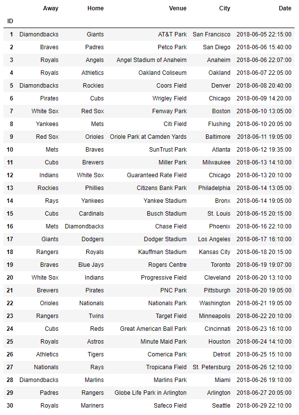
The optimal solution I obtained from the 11th experiment gives the best schedule time for the 2018 season, which is just over 24 days (24 days and 3 hours). The solution starts with Diamondbacks @ Giants in AT&T Park, San Francisco on the 5th of June and ends with Royals @ Mariners in Safeco Field, Seattle on the 29th of June. This is the global best solution among the scheduled games this season. Maps and itineraries of selected solutions are shown below. Click on any of the plots and tables to see the Jupyter notebook. All times in these schedules are in EDT.

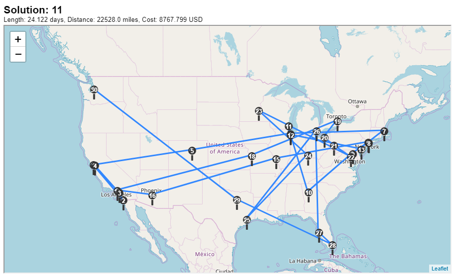
As a 22,528-mile trip, this schedule costs roughly $8,767. By changing the objective, it is possible to obtain a better cost, however the schedule takes longer significantly longer. Solution 12 is only 11,914 miles. It's 10,614 miles shorter and $2,149 cheaper compared to Solution 11 but takes 4 days longer.

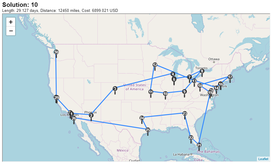
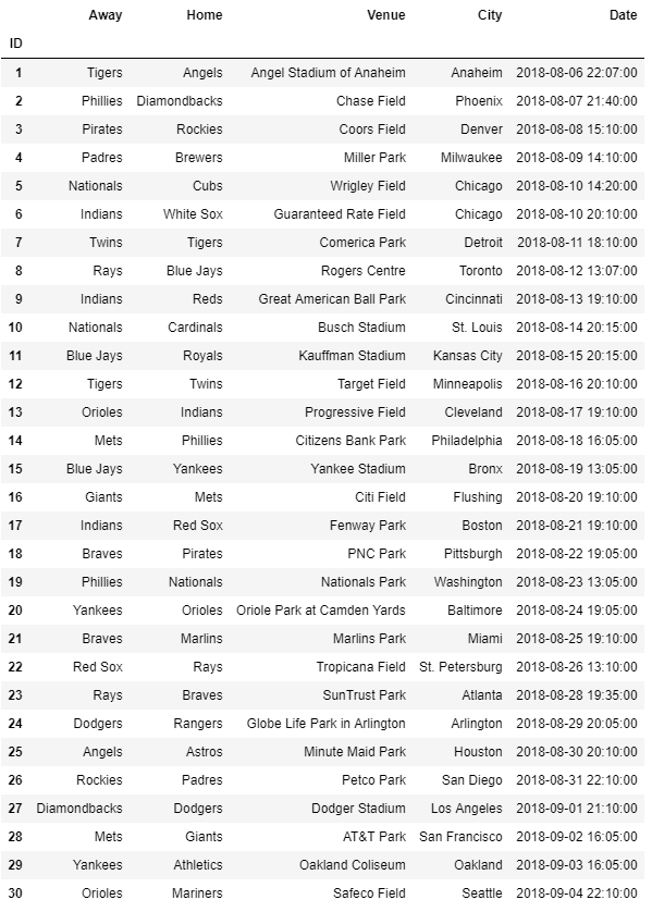
Among the schedules you can still try at the writing of this post, Solution 9 gives the shortest schedule time (24 days 3 hours) and Solution 10 gives the best cost ($6,899). The latter schedule starts with Tigers @ Angels in Angel Stadium, Anaheim on the 6th of August, and ends with Orioles @ Mariners in Safeco Field, Seattle on the 4th of September. Note that, this solution is the longest schedule among all solutions I have with a little over 29 days.

Here's a list of all solutions:

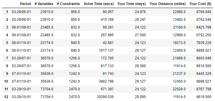
The objective and the time period of the formulation heavily affect the solution time. Minimizing the cost takes longer due to unique optimal solutions. Moreover, increasing the time period from 3 months to 6 months nearly quadruples the solution time.

Ultimately, the best trip is up to you. You can define another objective of your choice, whether it be minimizing the cost, minimizing the schedule time, avoiding the risky connections (minimum time between games minus the driving time), minimizing the total driving time, or even maximizing the landmarks you have visited along the way. Whatever objective you choose, you can use sasoptpy and use the powerful SAS Viya mixed integer linear optimization solver to generate a trip that is perfect for you! Working in Python allows you to integrate packages you are familiar with and makes everything smoother. Do not forget to check my Jupyter notebook and see the Python files.

Moving Further

You can further improve this model based on your desire. Here I list a few ideas:

If you would like to see an away and a home game for every team exactly once, then you can add the following constraint

$\displaystyle \sum_{(g, g_1) \in \text{ARCS}: \text{away}[g]= t \text{ and } \text{away}[g_1] \not = t} u[g,g_1]+\sum_{(g_1, g) \in \text{ARCS}: \text{away}[g]= t \text{ and } \text{away}[g_1] \not = t} u[g_1,g] = 1 \qquad \forall t \in \text{TEAMS}$

You can try to avoid risky connections you have in the schedule by replacing the objective with

$\displaystyle \text{maximize: } \sum_{(g_1,g_2) \in \text{ARCS}} ( \text{start}[g_2] - \text{end}[g_1] - c[g_1,g_2])\cdot u[g_1, g_2]$

To prevent schedules that are too long, you should add a limit to the total schedule length, for example, 25 days:

$\displaystyle \sum_{(g, \text{sink}) \in \text{ARCS}} \text{end}[g]\cdot u[g, \text{sink}] - \sum_{(\text{source}, g) \in \text{ARCS}} \text{start}[g]\cdot u[\text{source}, g] \leq 25$

Share how you define the perfect schedule below if you have more ideas!