It can be frustrating when the same probability distribution has two different parameterizations, but such is the life of a statistical programmer. I previously wrote an article about the gamma distribution, which has two common parameterizations: one that uses a scale parameter (β) and another that uses a rate parameter (c = 1/β).
The relationship between scale and rate parameters is straightforward, but sometimes the relationship between different parameterizations is more complicated. Recently, a SAS programmer was using a regression procedure to fit the parameters of a Weibull distribution. He was confused about how the output from a SAS regression procedure relates to a more familiar parameterization of the Weibull distribution, such as is fit by PROC UNIVARIATE. This article shows how to perform two-parameter Weibull regression in several SAS procedures, including PROC RELIABILITY, PROC LIFEREG, and PROC FMM. The parameter estimates from regression procedures are not the usual Weibull parameters, but you can transform them into the Weibull parameters.
This article fits a two-parameter Weibull model. In a two-parameter model, the threshold parameter is assumed to be 0. A zero threshold assumes that the data can be any positive value.
For other distributions, see the SAS Usage Note that shows how to transform regression estimates into the usual parameters in the RAND, PDF, and QUANTILE functions. You can use the Usage Note to transform many models that are fit in PROC GENMOD, GLIMMIX, and FMM. For example, the note shows how to transform estimates for Poisson regression, negative binomial regression, gamma regression, and Tweedie regression.
Fitting a Weibull distribution in PROC UNIVARIATE
PROC UNIVARIATE is the first tool to reach for if you want to fit a Weibull distribution in SAS.
The most common parameterization of the Weibull density is
\(f(x; \alpha, \beta) =
\frac{\alpha}{\beta^{\alpha}} (x)^{\alpha-1} \exp \left(-\left(\frac{x}{\beta}\right)^{\alpha }\right)\)
where
α is a shape parameter and β is a scale parameter. This parameterization is used by most Base SAS functions and procedures, as well as many regression procedures in SAS.
The following SAS DATA step simulates data from the Weibull(α=1.5, β=0.8) distribution and fits the parameters by using PROC UNIVARIATE:
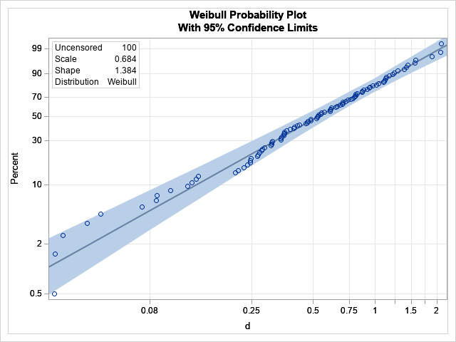
/* sample from a Weibull distribution */ %let N = 100; data Have(drop=i); call streaminit(12345); do i = 1 to &N; d = rand("Weibull", 1.5, 0.8); /* Shape=1.5; Scale=0.8 */ output; end; run; proc univariate data=Have; var d; histogram d / weibull endpoints=(0 to 2.5 by 0.25); /* fit Weib(Sigma, C) to the data */ probplot / weibull2(C=1.383539 SCALE=0.684287) grid; /* OPTIONAL: P-P plot */ ods select Histogram ParameterEstimates ProbPlot; run; |
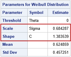
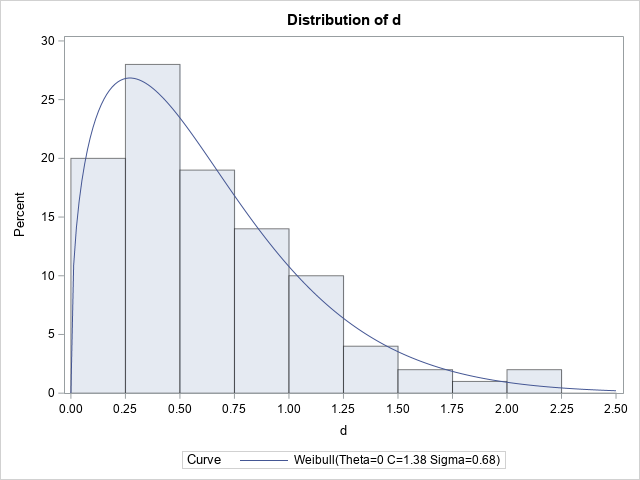
The histogram of the simulated data is overlaid with a density from the fitted Weibull distribution. The parameter estimates are Shape=1.38 and Scale=0.68, which are close to the parameter values. PROC UNIVARIATE uses the symbols c and σ for the shape and scale parameters, respectively.
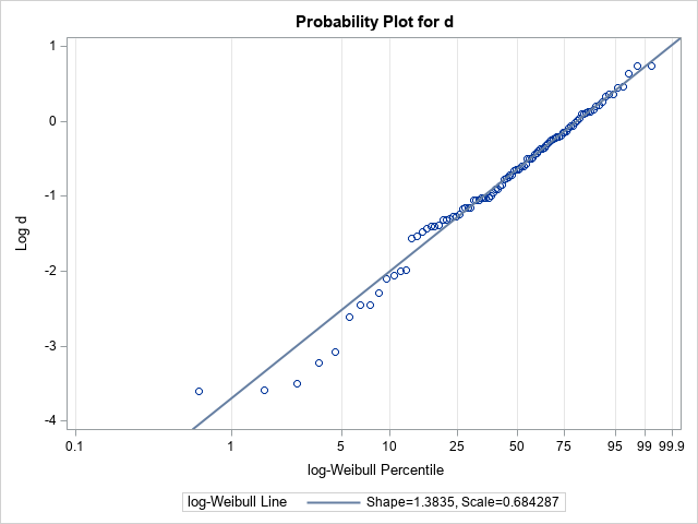
The probability-probability (P-P) plot for the Weibull distribution is shown. In the P-P plot, a reference line is added by using the option weibull2(C=1.383539 SCALE=0.684287). (In practice, you must run the procedure once to get those estimates, then a second time to plot the P-P plot.) The slope of the reference line is 1/Shape = 0.72 and the intercept of the reference line is log(Scale) = -0.38. Notice that the P-P plot is plotting the quantiles of log(d), not of d itself.
Weibull regression versus univariate fit
It might seem strange to use a regression procedure to fit a univariate distribution, but as I have explained before, there are many situations for which a regression procedure is a good choice for performing a univariate analysis. Several SAS regression parameters can fit Weibull models. In these models, it is usually assumed that the response variable is a time until some event happens (such as failure, death, or occurrence of a disease). The documentation for PROC LIFEREG provides an overview of fitting a model where the logarithm of the random errors follows a Weibull distribution. In this article, we do not use any covariates. We simply model the mean and scale of the response variable.
A problem with using a regression procedure is that a regression model provides estimates for intercepts, slopes, and scales. It is not always intuitive to see how those regression estimates relate to the more familiar parameters for the probability distribution. However, the P-P plot in the previous section shows how intercepts and slopes can be related to parameters of a distribution. The documentation for the LIFEREG procedure states that the Weibull scale parameter is exp(Intercept) and the Weibull shape parameter is the reciprocal of the regression scale parameter.
Notice how confusing this is! For the Weibull distribution, the regression model estimates a SCALE parameter for the error distribution. But the reciprocal of that scale estimate is the Weibull SHAPE parameter, NOT the Weibull scale parameter! (In this article, the response distribution and the error distribution are the same.)
Weibull regression in SAS
The LIFEREG procedure includes an option to produce a probability-probability (P-P) plot, which is similar to a Q-Q plot. The LIFEREG procedure also estimates not only the regression parameters but also provides estimates for the exp(Intercept) and 1/Scale quantities. The following statements use a Weibull regression model to fit the simulated data:
title "Weibull Estimates from LIFEREG Procedure"; proc lifereg data=Have; model d = / dist=Weibull; probplot; inset; run; |
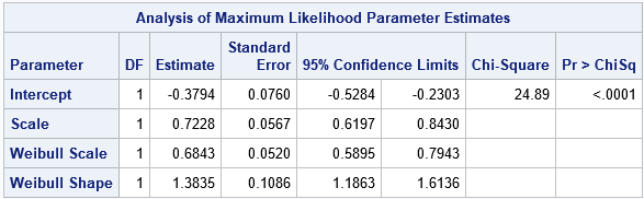
The ParameterEstimates table shows the estimates for the Intercept (-0.38) and Scale (0.72) parameters in the Weibull regression model. We previously saw these numbers as the parameters of the reference line in the P-P plot from PROC UNIVARIATE. Here, they are the result of a maximum likelihood estimate for the regression model. To get from these values to the Weibull parameter estimates, you need to compute Weib_Scale = exp(Intercept) = 0.68 and Weib_Shape = 1/Scale = 1.38. PROC LIFEREG estimates these quantities for you and provides standard errors and confidence intervals.
The graphical output of the PROBPLOT statement is equivalent to the P-P plot in PROC UNIVARIATE, except that PROC LIFEREG reverses the axes and automatically adds the reference line and a confidence band.
Other regression procedures
Before ending this article, I want to mention two other regression procedures that perform similar computations: PROC RELIABILITY, which is in SAS/QC software, and PROC FMM in SAS/STAT software.
The following statements call PROC RELIABILITY to fit a regression model to the simulated data:
title "Weibull Estimates from RELIABILITY Procedure"; proc reliability data=Have; distribution Weibull; model d = ; run; |
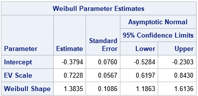
The parameter estimates are similar to the estimates from PROC LIFEREG. The output also includes an estimate of the Weibull shape parameter, which is 1/EV_Scale. The output does not include an estimate for the Weibull scale parameter, which is exp(Intercept).
In a similar way, you can use PROC FMM to fit a Weibull model. PROC FMM Is typically used to fix a mixture distribution, but you can specify the K=1 option to fit a single response distribution, as follows:
title "Weibull Estimates from FMM Procedure"; proc fmm data=Have; model d = / dist=weibull link=log k=1; ods select ParameterEstimates; run; |
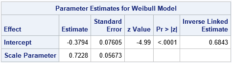
The ParameterEstimates table shows the estimates for the Intercept (-0.38) and Scale (0.72) parameters in the Weibull regression model. The Weibull scale parameter is shown in the column labeled "Inverse Linked Estimate." (The model uses a LOG link, so the inverse link is EXP.) There is no estimate for the Weibull shape parameter. which is the reciprocal of the Scale estimate.
Summary
The easiest way to fit a Weibull distribution to univariate data is to use the UNIVARIATE procedure in Base SAS. The Weibull shape and scale parameters are directly estimated by that procedure. However, you can also fit a Weibull model by using a SAS regression procedure. If you do this, the regression parameters are the Intercept and the scale of the error distribution. You can transform these estimates into estimates for the Weibull shape and scale parameters. This article shows the output (and how to interpret it) for several SAS procedures that can fit a Weibull regression model.
Why would you want to use a regression procedure instead of PROC UNIVARIATE? One reason is that the response variable (failure or survival) might depend on additional covariates. A regression model enables you to account for additional covariates and still understand the underlying distribution of the random errors. A second reason is that the FMM procedure can fit a mixture of distributions. To make sense of the results, you must be able to interpret the regression output in terms of the usual parameters for the probability distributions. In a second article, I show how to fit a mixture of Weibull distributions.

13 Comments
Pingback: Fit a mixture of Weibull distributions in SAS - The DO Loop
Nice article Rick. By the way, PROC SEVERITY also fits the Weibull.
proc severity data=Have;
loss d;
dist weibull;
run;
Dear Rick,
thank you for posting this. I love parametric models for survival analysis, I feel that they deserve much more attention in the applied statistics community.
I once played around with the (sparsely documented ...) automatic variable _LOGL_ in GLIMMIX which allows defining the LogLikelihood function. If you additionally define the automatic scale parameter _PHI_ to be the _VARIANCE_ then you can come up with the following GLIMMIX code for a Weibull model. Having the model in GLIMMIX is nice because you have access to the various options of the procedure, e.g., fitting correlated observations via the RANDOM statement.
Yours,
Oliver
title "Weibull Estimates from GLIMMIX Procedure";
proc glimmix data=Have;
model d = / s;
rho = exp(-_linp_);
_variance_=_phi_;
_logl_= log(_phi_*rho*((rho*d)**(_phi_-1)) * exp(-(rho*d)**_phi_));
run;
Dear Rick,
Thanks for the post. I have a question related to Weibull fitting. I have 5 Cumulative Probability of Default (CPD) points for five years. How can I use Weibull Distribution to forecast following 10 years?
I have checked other platforms too but couldn't find the solution.
Kind Regards,
Just five points? Your model might not be very accurate.
I suspect this question will require several back-and-forth interactions and posting sample data and SAS code. Please post to the SAS Support Communities if you want a SAS solution.
Thanks for your reply.
Truth is I tried polynomial functions and their fitting was quiet accurate. However, I received feedback that I should be using weibull distribution. Thus, I will post on SAS community.
Thanks again,
Kind Regards.
Hi Rick,
First thank you for the detailed analysis on the different ways to model weibulls. A lot of times we get mixed mode data (failures and suspensions) where we don't know the specific failure mode. Is there a way bring censored data (failures and suspension times) into proc fmm? I want to run a mixed mode weibull (not on a mixed distribution but mixed failure/ suspension data). I don't see where censor information can be added to the model.
Thanks
Mark
Mark,
The FMM procedure does not currently support censoring. You can use the RELIABILITY procedure if you want to include censoring in a Weibull analysis, but of course that procedure does not support mixture models.
Best,
Dave
Hello Rick,
Thank you for this helpful posting. This helps a lot to clear some concerns regarding the parametrization of Weibull distribution that SAS is using.
I had one simple question though. Would you clarify if it's alpha as shape parameter and beta as scale parameter (right below the distribution specification), or have they been swapped?
Thank you,
Soo
Thank you for your careful reading. Yes, in the formula I originally swapped the meaning of alpha and beta. I have fixed the error, so refresh your browser cache.
Dear Rick,
Thank you for your prompt response on my previous question. The update you made cleared up the concern. Thank you.
If you don't mind me asking, does Weibull AFT model parametrization in PROC LIFEREG involve any kind of transformation of the parameters that are being estimated, such as R does given in this documentation (https://cran.r-project.org/web/packages/SurvRegCensCov/vignettes/weibull.pdf)?
I've been trying to figure out interchangeability between model formulation (log linear model) vs. likelihood construction ((hazard^indicator)*survival) of Weibull AFT model for a survival outcome.
I didn't think I saw any detail regarding this within SAS documentation for PROC LIFEREG. Would much appreciate if you have any thoughts to share on this matter.
Thank you,
Soo Kyung
If it is not mentioned in the doc, you can ask Technical Support.
Hmmm, interesting. I wonder how to get the hazard ratio and its confidence interval from the PROC LIFEREG procedure with a Weibull distribution. The HR must be constant, as same to the Cox model.