The field of probability and statistics is full of asymptotic results. The Law of Large Numbers and the Central Limit Theorem are two famous examples. An asymptotic result can be both a blessing and a curse. For example, consider a result that says that the distribution of some statistic converges to the normal distribution as the sample size goes to infinity. This is a blessing because it means that you can estimate standard errors and confidence intervals for the statistic by applying simple formulas from the normal distribution. However, when I use an asymptotic approximation, I always hear a little voice in my head that whispers, "Are you sure the sample size is sufficiently large?"
One way to quiet that voice is to use a simulation to explore how large the sample must be before an asymptotic result becomes valid in practice. For some asymptotic results, textbooks give guidance about when the asymptotic result is valid. For example, many undergraduate texts recommend N ≥ 30 as a cutoff at which the Central Limit Theorem (CLT) applies, regardless of the shape of the underlying distribution. The Wikipedia article on the Central Limit Theorem shows several simulations that demonstrate the CLT.
This article examines a question that a reader asked on my blog. Recall that for normally distributed data X ~ N(μ, σ), you can use the sample mean, standard deviation, and sample size to estimate a confidence interval for the mean. The endpoints of the interval estimate are \(\bar{x} \pm t_{1-\alpha/2, N-1} \, s/\sqrt{N}\), where \(t_{1-\alpha/2, N-1}\) is a critical quantile from the t distribution with N-1 degrees of freedom. The reader asked when this formula is valid for statistics that are asymptotically normal. This article shows how to use simulation in SAS to answer questions like this on a case-by-case basis.
The distribution of the sample mean of ChiSq(k)
The question concerns confidence intervals for the mean of a chi-square distribution with k degrees of freedom. How large does the sample size have to be before you can use the asymptotic formula for a (normal) confidence interval?
The Central Limit Theorem applies to this case, so you can assume that the formula is approximately valid for a sample of size N ≥ 30. But what does "approximately valid" mean? And if you use the normal-based formula on smaller samples, is the result approximately correct, or is it way off? The next section demonstrates how to answer these questions by using a simulation study.
A simulation to reveal an asymptotic result
This section shows how to use a simulation to investigate when the normal-based formula for a 95% confidence interval is a good estimate for the true confidence interval. This section follows the techniques in the article "Coverage probability of confidence intervals: A simulation approach." If you have not previously performed a simulation to determine confidence intervals, start by reading that article, which explains the fundamental ideas.
When you conduct a simulation study, it is best to write down what you are simulating, from what distribution, and what you are trying to investigate. The following pseudocode specifies the simulation for this example:
For each parameter value k=10, 20, ... do the following steps:
    For sample sizes N=2, 3, ..., 40, do the following steps:
        Generate 10,000 samples of size N from the chi-square distribution with k degrees of freedom.
            For each sample:
                Compute the sample mean and standard deviation.
                Use them in the formula for the normal confidence interval.
                Determine whether the confidence interval contains the true mean of the
                          ChiSquare(k) distribution, which is k.
        Estimate the coverage probability as the proportion of samples for which the
confidence interval contains the true mean. |
In a previous article, I showed "how to perform this simulation study by using the SAS DATA step and Base SAS procedures. For comparison, the following program implements the simulation by using the SAS/IML matrix language. For simplicity, I do not loop over the degrees of freedom, but hard-code k=20 degrees of freedom.
%let DF = 20; /* degrees of freedom parameter */ %let NumSamples = 10000; /* number of samples in each simulation */ proc iml; k = &DF; call randseed(12345); Sizes = 2:40; /* sample sizes */ /* allocate the results matrix */ varNames = {'N' 'Coverage'}; h = ncol(varNames); results = j(ncol(Sizes), h, .); results[,1] = Sizes`; do i = 1 to ncol(Sizes); N = Sizes[i]; mu = k; /* true mean of chi-square(k) distribution */ x = j(N, &NumSamples, .); /* N x NumSamples matrix */ call randgen(x, "chisq", k); /* fill each column with chi-square(k) variates */ /* use the normal formula to estimate CIs from samples */ SampleMean = mean(x); /* compute sample mean and standard error */ SampleSEM = std(x) / sqrt(n); tCrit = quantile("t", 1-0.05/2, N-1); /* two-sided critical value of t statistic, alpha=0.05 */ Lower = SampleMean - tCrit*SampleSEM; Upper = SampleMean + tCrit*SampleSEM; /* what proportion of CIs contain the true mean? */ ParamInCI = (Lower<mu & Upper>mu); /* indicator variable */ prop = mean(ParamInCI`); results[i,2] = prop; end; create MCResults from results[c=VarNames]; append from results; close; QUIT; title "Empirical Coverage of Confidence Intervals"; title2 "X ~ Chi-Square(&DF)"; proc sgplot data=MCResults; scatter x=N y=Coverage; refline 0.95 / axis=y noclip; label N="Sample Size (N)" Coverage="Empirical Coverage Probability"; run; |
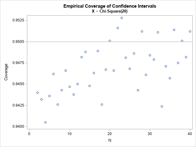
The graph shows the empirical coverage probability for each value of the sample size, N. For k=20 degrees of freedom, the coverage probability appears to be less than 95% for very small samples but increases towards 95% as the sample size grows.
You can change the value of the DF macro variable to see how the graph changes for other values of the degrees-of-freedom parameter. The following graph shows the coverage probability for k=10 degrees of freedom and for a range of sample sizes. If you use the CI formula that is based on the assumption of normality, you will be slightly overconfident. The nominal "95% CI" is more like a 93% or 94% CI for small samples from the chi-square(10) distribution. Of course, you could adjust for this by increasing the confidence level that is used in the normal-based formula. For example, you might want to use the formula for a nominal 96% CI to ensure that the coverage probability for small samples is at least 95% in practice.
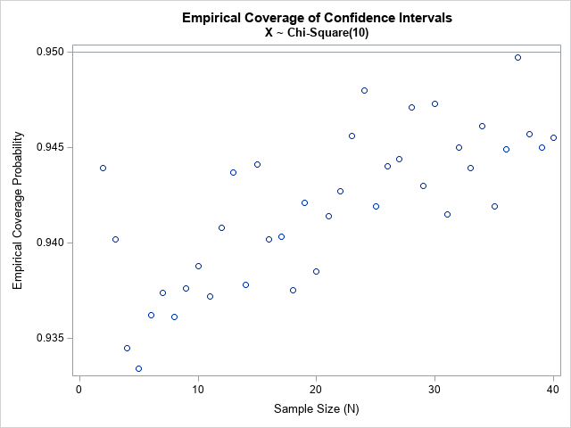
Notice in both graphs that the coverage probability is close to 95% for samples sizes N ≥ 30. You can see the Central Limit Theorem kicking in! The simulation study enables you to quantify this asymptotic result and to determine whether N ≥ 30 is "sufficiently large" for whatever asymptotic result you are considering using. You can modify the program and convince yourself that N ≥ 60 might be a safer choice when k=10.
Summary
In summary, simulation studies are useful for investigating whether an asymptotic result is valid for the sample sizes that you want to analyze. This article examined the question of whether you can use a normal-based formula to estimate the confidence interval for a mean. The Central Limit Theorem says that you do this for "sufficiently large" samples, but what does that mean in practice? A Monte Carlo simulation study enables you to quantify that statement. You can estimate the empirical coverage probability when you apply the formula to small sample sizes. This article used a SAS/IML program to implement the simulation study, but you could also use the SAS DATA step and Base SAS procedures, as shown in a previous article.
