This article uses simulation to demonstrate the fact that any continuous distribution can be transformed into the uniform distribution on (0,1). The function that performs this transformation is a familiar one: it is the cumulative distribution function (CDF). A continuous CDF is defined as an integral, so the transformation is called the probability integral transformation.
This article demonstrates the probability integral transformation and its close relative, the inverse CDF transformation. These transformations are useful in many applications, such as constructing statistical tests and simulating data.
The probability integral transform
Let X be a continuous random variable whose probability density function is f. Then the corresponding cumulative distribution function (CDF) is the integral \(F(x) = \int\nolimits_{-\infty}^{x} f(t)\,dt\). You can prove that the random variable Y = F(X) is uniformly distributed on (0,1). In terms of data, if {X1, X2, ..., Xn} is a random sample from X, the values {F(X1), F(X2), ..., F(Xn)} are a random sample from the uniform distribution.
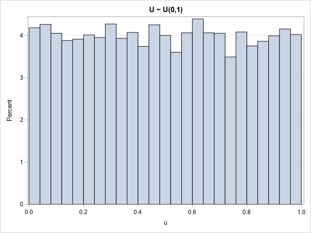
Let's look at an example. The following SAS DATA step generates a random sample from the Gamma distribution with shape parameter α=4. At the same time, the DATA step computes U=F(X), where F is the CDF of the gamma distribution. A histogram of the U variable shows that it is uniformly distributed:
/* The probability integral transformation: If X is a random variable with CDF F, then Y=F(X) is uniformly distributed on (0,1). */ %let N = 10000; data Gamma4(drop=i); call streaminit(1234); do i = 1 to &N; x = rand("Gamma", 4); /* X ~ Gamma(4) */ u = cdf("Gamma", x, 4); /* U = F(X) ~ U(0,1) */ output; end; run; title "U ~ U(0,1)"; proc sgplot data=Gamma4; histogram U / binwidth=0.04 binstart=0.02; /* center first bin at h/2 */ yaxis grid; run; |

The histogram has some bars that are greater than the average and others that are less than the average. That is expected in a random sample.
One application of the CDF transformation is to test whether a random sample comes from a particular distribution. You can transform the sample by using the CDF function, then test whether the transformed values are distributed uniformly at random. If the transformed variates are uniformly distributed, then the original data was distributed according to the distribution F.
The inverse probability transformation
It is also useful to run the CDF transform in reverse. That is, start with a random uniform sample and apply the inverse-CDF function (the quantile function) to generate random variates from the specified distribution. This "inverse CDF method" is a standard technique for generating random samples.
The following example shows how it works. The DATA step generates random uniform variates on (0,1). The variates are transformed by using the quantiles of the lognormal(0.5, 0.8) distribution. A call to PROC UNIVARIATE overlays the density curve of the lognormal(0.5, 0.8) distribution on the histogram of the simulated data. The curve matches the data well:
/* inverse probability transformation */ data LN(drop=i); call streaminit(12345); do i = 1 to &N; u = rand("Uniform"); /* U ~ U(0,1) */ x = quantile("Lognormal", u, 0.5, 0.8); /* X ~ LogNormal(0.5, 0.8) */ output; end; run; proc univariate data=LN; var x; histogram x / lognormal(scale=0.5 shape=0.8) odstitle="X ~ LogNormal(0.5, 0.8)"; run; |

Summary
The probability integral transform (also called the CDF transform) is a way to transform a random sample from any distribution into the uniform distribution on (0,1). The inverse CDF transform transforms uniform data into a specified distribution. These transformations are used in testing distributions and in generating simulated data.
Appendix: Histograms of uniform variables
The observant reader might have noticed that I used the BINWIDTH= and BINSTART= options to set the endpoints of the bin for the histogram of uniform data on (0,1). Why? Because by default the histogram centers bins. For data that are bounded on an interval, you can use the BINWIDTH= and BINSTART= options to improve the visualization.
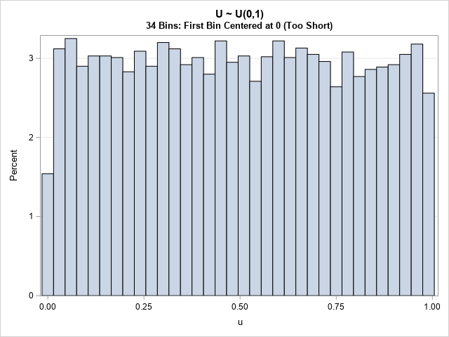
Let's use the default binning algorithm to create a histogram of the uniform data:
title "U ~ U(0,1)"; title2 "34 Bins: First Bin Centered at 0 (Too Short)"; proc sgplot data=Gamma4; histogram u; yaxis grid; run; |

Notice that the first bin is "too short." The first bin is centered at the location U=0. Because the data cannot be less than 0, the first bin has only half as many counts as the other bins. The last bin is also affected, although the effect is not usually as dramatic.
The histogram that uses the default binning is not wrong, but it doesn't show the uniformity of the data as clearly as a histogram that uses the BINWIDTH= and BINSTART= options to force 0 and 1 to be the endpoints of the bins.

1 Comment
Pingback: An introduction to simulating correlated data by using copulas - The DO Loop