As mentioned in my article about Monte Carlo estimate of (one-dimensional) integrals, one of the advantages of Monte Carlo integration is that you can perform multivariate integrals on complicated regions. This article demonstrates how to use SAS to obtain a Monte Carlo estimate of a double integral over rectangular and non-rectangular regions. Be aware that a Monte Carlo estimate is often less precise than a numerical integration of the iterated integral.
Monte Carlo estimate of multivariate integrals
Multivariate integrals are notoriously difficult to solve. But if you use Monte Carlo methods, higher-dimensional integrals are only marginally more difficult than one-dimensional integrals. For simplicity, suppose we are interested in the double integral \(\int_D f(x,y) \,dx\,dy\), where D is a region in the plane. The basic steps for estimating a multivariate integral are as follows:
- Generate a large random sample of points from the uniform distribution on the domain, D.
- Evaluate f at each point (x,y) in the random sample. Let W = f(X,Y) be the vector of values.
- Compute Area(D)*mean(W), where Area(D) is the area of D and mean(W) is the arithmetic average of W. If you know the exact area of D, use it. If D is a very complicated shape, you can estimate the area of D by using the Monte Carlo methods in this article.
The quantity Area(D)*mean(W) is a Monte Carlo estimate of \(\int_D f(x,y) \,dx\,dy\). The estimate depends on the size of random sample (larger samples tend to give better estimates) and the particular random variates in the sample.
Monte Carlo estimates of double integrals on rectangular regions
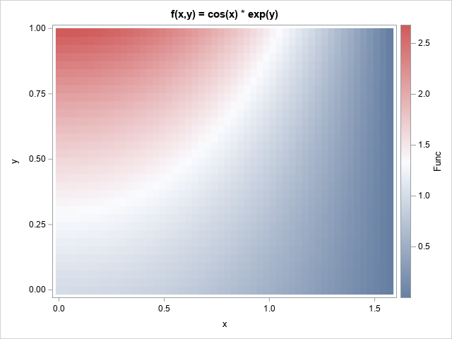
Let's start with the simplest case, which is when the domain of integration, D, is a rectangular region. This section estimates the double integral of f(x,y) = cos(x)*exp(y) over the region D = [0,π/2] x [0,1]. That is, we want to estimate the integral
\(\int\nolimits_0^{\pi/2}\int\nolimits_0^1 \cos(x)\exp(y)\,dy\,dx = e - 1 \approx 1.71828\)
where e is the base of the natural logarithm. For this problem, the area of D is (b-a)*(d-c) = π/2.
The graph at the right shows a heat map of the function on the rectangular domain.
The following SAS/IML program defines the integrand and the domain of integration. The program generates 5E6 uniform random variates on the interval [a,b]=[0,π/2] and on the interval [c,d] = [0,1]. The (x,y) pairs are evaluated, and the vector W holds the result. The Monte Carlo estimate is the area of the rectangular domain times the mean of W:
/* Monte Carlo approximation of a double integral over a rectangular region */ proc iml; /* define integrand: f(x,y) = cos(x)*exp(y) */ start func(x); return cos(x[,1]) # exp(x[,2]); finish; /* Domain of integration: D = [a,b] x [c,d] */ pi = constant('pi'); a = 0; b = pi/2; /* 0 < x < pi/2 */ c = 0; d = 1; /* 0 < y < 1 */ call randseed(1234); N = 5E6; X = j(N,2); /* X ~ U(D) */ z = j(N,1); call randgen(z, "uniform", a, b); /* z ~ U(a,b) */ X[,1] = z; call randgen(z, "uniform", c, d); /* z ~ U(c,d) */ X[,2] = z; W = func(X); /* W = f(X1,X2) */ Area = (b-a)*(d-c); /* area of rectangular region */ MCEst = Area * mean(W); /* MC estimate of double integral */ /* the double integral is separable; solve exactly */ Exact = (sin(b)-sin(a))*(exp(d)-exp(c)); Diff = Exact - MCEst; print Exact MCEst Diff; |
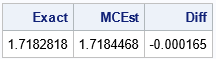
The output shows that the Monte Carlo estimate is a good approximation to the exact value of the double integral. For this random sample, the estimate is within 0.0002 units of the true value.
Monte Carlo estimates of double integrals on non-rectangular regions
It is only slightly more difficult to estimate a double integral on a non-rectangular domain, D. It is helpful to split the problem into two subproblems: (1) generate point uniformly in D, and (2) estimate the integral on D.
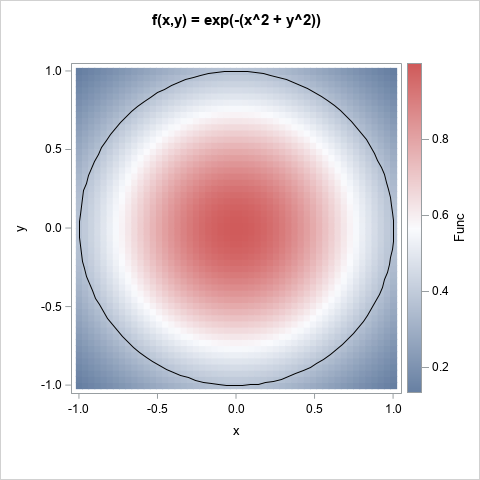
The next two sections show how to estimate the integral of f(x,y) = exp(-(x2 + y2)) over the circle of unit radius centered at the origin: D = {(x,y) | x2 + y2 ≤ 1}. The graph at the right shows a heat map of the function on a square. The domain of integration is the unit disk.
By using polar coordinates, you can solve this integral exactly. The double integral has the value 2π*(e – 1)/(2 e) ≈ 1.9858653, where e is the base of the natural logarithm.
Generate point uniformly in a non-rectangular planar region
For certain shapes, you can directly generate a random sample of uniformly distributed points:
- You can generate a uniform random sample in a planar disk.
- You can generate a uniform random sample in any triangle and in any planar region that can be decomposed into a union of triangles.
In general, for any planar region, you can use the acceptance-rejection technique. I previously showed an example of using Monte Carlo integration to estimate π by estimating the area of a circle.
Because the acceptance-rejection technique is the most general, let's use it to generate a random set of points in the unit disk, D. The steps are as follows:- Construct a bounding rectangle for the region. In this example, you can use R = [-1,1] x [-1,1].
- Generate random points uniformly at random in the rectangle.
- Keep the points that are in the domain, D. Discard the others.
If you know the area of D, you can use a useful trick to choose the sample size. When you use an acceptance-rejection technique, you do not know in advance how many points will end up in D. However, you can estimate the number as ND ≈ NR*Area(D)/Area(R), where NR is the sample size in R. If you know the area of D, you can invert this formula. If you want approximately ND points to be in D, generate ND*Area(R)/Area(D) points in R. For example, suppose you want ND=5E6 points in the unit disk, D. We can choose NR ≥ ND*4/π, as in the following SAS/IML program, which generates random points in the unit disk:
proc iml; /* (1) Generate approx N_D points in U(D), where D is the unit disk D = { (x,y) | x**2 + y**2 <= 1 } */ N_D = 5E6; /* we want this many points in D */ a = -1; b = 1; /* Bounding rectangle, R: */ c = -1; d = 1; /* R = [a,b] x [c,d] */ /* generate points inside R. Generate enough points (N_R) in R so that approximately N_D are actually in D */ pi = constant('pi'); area_Rect = (b-a)*(d-c); area_D = pi; N_R = ceil(N_D * area_Rect / area_D); /* estimate how many points in R we'll need */ call randseed(1234); X = j(N_R,2); z = j(N_R,1); call randgen(z, "uniform", a, b); X[,1] = z; call randgen(z, "uniform", c, d); X[,2] = z; /* which points in the bounding rectangle are in D? */ b = (X[,##] <= 1); /* x^2+y^2 <= 1 */ X = X[ loc(b),]; /* these points are in D */ print N_D[L="Target N_D" F=comma10.] (nrow(X))[L="Actual N_D" F=comma10.]; |
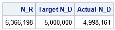
The table shows the result. The program generated 6.3 million points in the rectangle, R. Of these, 4.998 million were in the unit disk, D. This is very close to the desired number of points in D, which was 5 million.
Monte Carlo estimate of an integral over a planar region
Each row of the matrix, X, contains a point in the disk, D. The points are a random sample from the uniform distribution on D. Therefore, you can estimate the integral by calculating the mean value of the function on these points:
/* (2) Monte Carlo approximation of a double integral over a non-rectangular domain. Estimate integral of f(x,y) = exp(-(x**2 + y**2)) over the disk D = { (x,y) | x**2 + y**2 <= 1 } */ /* integrand: f(x,y) = exp(-(x**2 + y**2)) */ start func(x); r2 = x[,1]##2 + x[,2]##2; return exp(-r2); finish; W = func(X); MCEst = Area_D * mean(W); /* compare the estimate to the exact value of the integral */ e = constant('e'); Exact = 2*pi*(e-1)/(2*e); Diff = Exact - MCEst; print Exact MCEst Diff; |
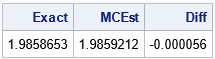
The computation shows that a Monte Carlo estimate of the integral over the unit disk is very close to the exact value. For this random sample, the estimate is within 0.00006 units of the true value.
Summary
This article shows how to use SAS to compute Monte Carlo estimates of double integrals on a planar region. The first example shows a Monte Carlo integration over a rectangular domain. The second example shows a Monte Carlo integration over a non-rectangular domain. For a non-rectangular domain, the integration requires two steps: first, use an acceptance-rejection technique to generate points uniformly at random in the domain; then use Monte Carlo to estimate the integral. The technique in this article generalizes to integration on higher-dimensional domains.

1 Comment
Pingback: Top 10 posts from The DO Loop in 2021 - The DO Loop