A previous article shows how to use Monte Carlo simulation to estimate a one-dimensional integral on a finite interval. A larger random sample will (on average) result in an estimate that is closer to the true value of the integral than a smaller sample. This article shows how you can determine a sample size so that the Monte Carlo estimate is within a specified distance from the true value, with high probability.
This article is inspired by and uses some of the notation from Neal, D. (1983) "Determining Sample Sizes for Monte Carlo Integration," The College Mathematics Journal.
Ensure the estimate is (probably) close to the true value
As shown in the previous article, a Monte Carlo estimate of an integral of g(x) on the interval (a,b) requires three steps:
- Generate a uniform random sample of size n on (a,b). Let X be the vector of n uniform random variates.
- Use the function g to evaluate each point in the sample. Let Y = g(X) be the vector of transformed variates.
- An estimate of the integral \(\int\nolimits_{a}^{b} g(x) \, dx\) is (b - a)*mean(Y), where mean(Y) is the arithmetic average of Y, as shown in the previous article.
The goal of this article is to choose n large enough so that, with probability at least β, the Monte Carlo estimate of the integral
is within δ of the true value.
The mathematical derivation is at the end of this article. The result (Neal, 1983, p. 257) is that you should choose
\(n > \left( \Phi^{-1}\left( \frac{\beta+1}{2} \right) \frac{(b-a)s_{Y}}{\delta} \right)^2\)
where \(\Phi^{-1}\) is the quantile function of the standard normal distribution, and \(s_{Y}\) is an estimate of the standard deviation of Y.
Applying the formula to a Monte Carlo estimate of an integral
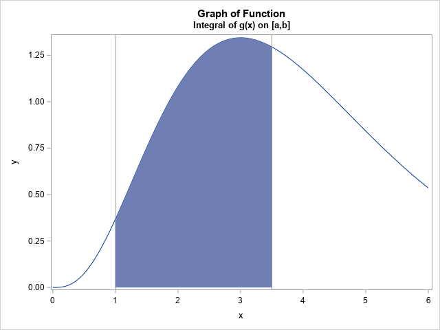
Let's apply the formula to see how large a sample size we need to estimate the integral \(\int\nolimits_{a}^{b} g(x) \, dx\) to three decimal places (δ=5E-4) for the function g(x) = xα-1 exp(-x), where α=4 and the interval of integration is (1, 3.5). The function is shown at the top of this article.
The estimate requires knowing an estimate for the standard deviation of Y=g(X), where X ~ U(a,b). You can use a small "pilot study" to obtain the standard deviation, as shown in the following SAS/IML program. You could also use the DATA step and PROC MEANS for this computation.
%let alpha = 4; /* shape parameter */ %let a = 1; /* lower limit of integration */ %let b = 3.5; /* upper limit of integration */ proc iml; /* define the integrand */ start Func(x) global(shape); return x##(shape - 1) # exp(-x); finish; call randseed(1234); shape = α a = &a; b = &b; /* Small "pilot study" to estimate s_Y = stddev(Y) */ N = 1e4; /* small sample */ X = j(N,1); call randgen(x, "Uniform", a, b); /* X ~ U(a,b) */ Y = func(X); /* Y = f(X) */ s = std(Y); /* estimate of std dev(Y) */ |
For this problem, the estimate of the standard deviation of Y is about 0.3. For β=0.95, the value of \(\Phi^{-1}((\beta+1)/2) \approx 1.96\), but the following program implements the general formula for any probability, β:
/* find n so that MC est is within delta of true value with 95% prob */ beta = 0.95; delta = 5e-4; k = quantile("Normal", (beta+1)/2) * (b-a) * s; sqrtN = k / delta; roundN = round(sqrtN**2, 1000); /* round to nearest 1000 */ print beta delta roundN[F=comma10.]; |
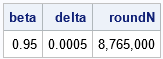
With 95% probability, if you use a sample size of n=8,765,000, the Monte Carlo estimate will be within δ=0.0005 units of the true value of the integral. Wow! That's a larger value than I expected!
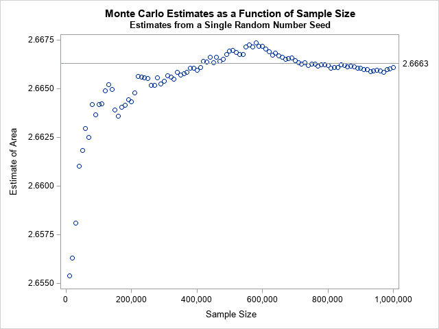
I used n=1E6 in the previous article and reported that the difference between the Monte Carlo approximation and the true value of the integral was less than 0.0002. So it is possible to be close to the true value by using a smaller value of n. In fact, the graph to the right (from the previous article) shows that for n=400,000 and n=750,000, the Monte Carlo estimate is very close for the specific random number seed that I used. But the formula in this section provides the sample size that you need to (probably!) be within ±0.0005 REGARDLESS of the random number seed.
The distribution of Monte Carlo estimates
I like to use SAS to check my math. The Monte Carlo estimate of the integral of g will vary according to the random sample. The math in the previous section states that if you generate k random samples of size n=8,765,000, that (on average) about 0.95*k of the sample will be within δ=0.0005 units of the true value of the integral, which is 2.666275. The following SAS/IML program generates k=200 random samples of size n and k estimates of the integral. We expect about 190 estimates to be within δ units of the true value and only about 10 to be farther away:
N = roundN; X = j(N,1); k = 200; Est = j(k,1); do i = 1 to k; call randgen(X, "Uniform", a, b); /* x[i] ~ U(a,b) */ Y = func(X); /* Y = f(X) */ f_avg = mean(Y); /* estimate E(Y) */ Est[i] = (b-a)*f_avg; /* estimate integral */ end; call quad(Exact, "Func", a||b); /* find the "exact" value of the integral */ Diff = Est - Exact; title "Difference Between Monte Carlo Estimate and True Value"; title2 "k=200 Estimates; n=8,765,000"; call Histogram(Diff) other="refline -0.0005 0.0005/axis=x;"; |
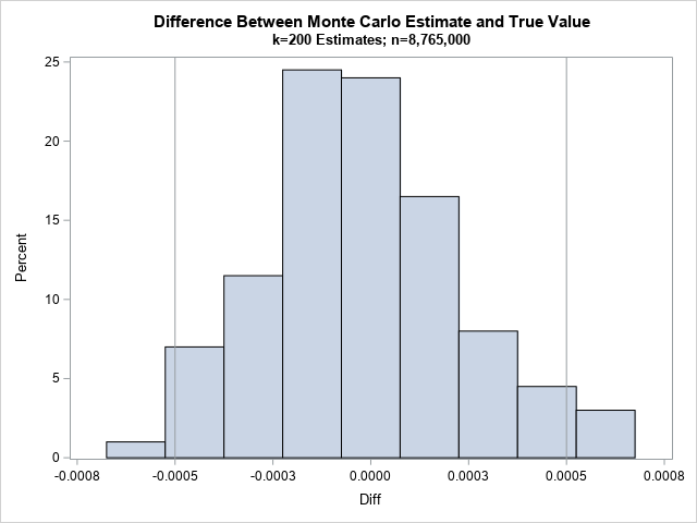
The histogram shows the difference between the exact integral and the estimates. The vertical reference lines are at ±0.0005. As predicted, most of the estimates are less than 0.0005 units from the exact value. What percentage? Let's find out:
/* how many estimates are within and NOT within delta? */ Close = ncol(loc(abs(Diff)<=delta)); /* number that are closer than delta to true value */ NotClose = ncol(loc(abs(Diff)> delta)); /* number that are farther than delta */ PctClose = Close / k; /* percent close to true value */ PctNotClose = NotClose / k; /* percent not close */ print k Close NotClose PctClose PctNotClose; |
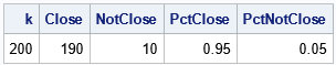
For this set of 200 random samples, exactly 95% of the estimates were accurate to within 0.0005. Usually, a simulation of 200 estimates would show that between 93% and 97% of the estimates are close. In this case, the answer was exactly 95%, but don't expect that to happen always!
Summary
This article shows how you can use elementary statistics to find a sample size that is large enough so that a Monte Carlo estimate is (probably!) within a certain distance of the exact value. The article was inspired by an article by Neal, D. (1983). The mathematical derivation of the result is provided in the next section.
Derivation of the sample size formula
This section derives the formula for choosing the sample size, n.
Because the Monte Carlo estimate is a mean, you can use elementary probability theory to find n.
Let {x1, x2, ..., xn} be random variates on (a, b). Let Y be the vector {g(x1), g(x2), ..., g(xn)}.
Let \(m_{n} = \frac{1}{n} \sum\nolimits_{i = 1}^{n} g(x_{i})\) be the mean of Y and let \(\mu = \frac{1}{b-a} \int\nolimits_{a}^{b} g(x) \, dx\) be the average value of g on the interval (a,b).
We know that \(m_n \to \mu\) as \(n \to \infty\). For any probability 0 < β < 1,
we want to find n large enough so that
\(P\left( | m_n - \mu | < \frac{\delta}{(b-a)} \right) \geq \beta\)
From the central limit theorem, we can substitute the standard normal random variable, Z, inside the parentheses by dividing by the standard error of Y, which is σY/sqrt(n):
\(P\left( | Z | < \frac{\delta \sqrt{n}}{(b-a)\sigma_{Y}} \right) \geq \beta\)
Equivalently,
\(2 P\left( Z < \frac{\delta \sqrt{n}}{(b-a)\sigma_{Y}} \right) - 1 \geq \beta\)
Solving the equation for sqrt(n) gives
\(\sqrt{n} > \Phi^{-1}\left( \frac{\beta+1}{2} \right) \frac{(b-a)\sigma_{Y}}{\delta}\)
Squaring both sides leads to the desired bound on n. Because we do not know the true standard deviation of Y, we substitute a sample statistic, sY.

2 Comments
hi Rick Wicklin! I would like to know how I can produce a geometric brownian motion using Proc IML or a data step. Could you help me?
The best place to get help with programming questions is the SAS Support Communities. I've written several articles that show how to simulate a random walk. The actual code you need depends on the dimensions of the problem (1-D, 2-D, etc) and the distribution that determines how the next location depends on the previous location. See some of these articles to get started:
Simulate a random walk (and the first comment)
The drunkard's walk in one dimension.
The drunkard's walk in two dimensions.