Numerical integration is important in many areas of applied mathematics and statistics. For one-dimensional integrals on the interval (a, b), SAS software provides two important tools for numerical integration:
- For common univariate probability distributions, you can use the CDF function to integrate the density, thus obtaining the probability that a random variable takes a value in (a, b).
- For an arbitrary function that is continuous on (a,b), you can use the QUAD function in SAS/IML to numerically integrate the function.
This article shows a third method to estimate an integral in SAS: Monte Carlo simulation.
How to use Monte Carlo simulation to estimate an integral
I previously showed an example of using Monte Carlo simulation to estimate the value of pi (π) by using the "average value method." This section presents the mathematics behind the Monte Carlo estimate of the integral.
The Monte Carlo technique takes advantage of a theorem in probability that is whimsically called the Law of the Unconscious Statistician. The theorem is basically the chain rule for integrals. If X is a continuous random variable and Y = g(X) is a random variable that is created by a continuous transformation (g) of X, then the expected value of Y is given by the following convolution:
\(E[Y] = E[g(X)] = \int g(x) f_{X}(x) \,dx\)
where \(f_{X}\) is the probability density function for X.
To apply the theorem, choose X to be a uniform random variable on the interval (a,b). The density function of X is therefore \(f_{X}(x) = 1/(b-a)\) if x is in (a,b) and 0 otherwise. Rearranging the equation gives
\(\int_{a}^{b} g(x) \,dx = (b - a) \cdot E[g(X)]\)
Consequently, to estimate the integral of a continuous function g on the interval (a,b), you need to estimate the expected value E[g(X)], where X ~ U(a,b). To do this, generate a uniform random sample in (a,b), evaluate g on each point in the sample, and take the arithmetic mean of those values. In symbols,
\(\int_{a}^{b} g(x) \,dx \approx (b - a) \cdot \frac{1}{n} \sum\nolimits_{i = 1}^{n} g(x_{i})\)
where the \(x_i\) are independent random uniform variates on (a,b).
Estimate an integral in SAS by using Monte Carlo simulation
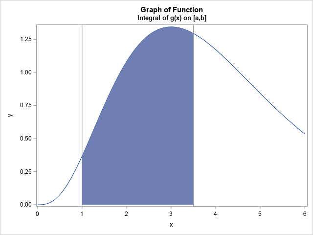
Suppose you want to estimate the integral of \(g(x) = x^{\alpha - 1} \exp(-x)\) on the interval (a,b) = (1, 3.5). The figure at the top of this article shows the graph of g for α=4 and the area under the curve on the interval (1, 3.5).
As mentioned earlier, an accurate way to numerically integrate the function is to use the QUAD subroutine in SAS/IML, as follows:
%let alpha = 4; /* shape parameter */ %let a = 1; /* lower limit of integration */ %let b = 3.5; /* upper limit of integration */ proc iml; /* define the integrand */ start Func(x) global(shape); return x##(shape - 1) # exp(-x); finish; /* call the QUAD subroutine to perform numerical integration */ shape = α a= &a; b = &b; call quad(AreaQuad, "Func", a||b); print AreaQuad; |

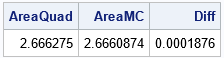
The QUAD subroutine approximates the area under the curve as 2.6663. This is a very accurate result. When you compute a Monte Carlo estimate, the estimate will depend on the size of the random sample that you use and the random number seed. The following SAS/IML program samples one million random variates from the uniform distribution on [1, 3.5]. The vector Y contains the transformed points (Y=g(X)). The call to the MEAN function estimates the expected value of g(x) when 1 < x < 3.5. If you multiply the mean by (3.5 - 1) = 2.5, you obtain an estimate of the integral, as follows:
/* Monte Carlo estimation of the integral */ call randseed(1234); N = 1e6; /* sample size for MC estimate */ X = j(N,1); /* allocate vector of size N */ call randgen(X, "Uniform", a, b); /* x[i] ~ U(a,b) */ Y = func(X); /* Y = f(X) */ f_avg = mean(Y); /* estimate E(Y) */ AreaMC = (b-a)*f_avg; /* estimate integral on (a,b) */ Diff = abs(AreaMC - AreaQuad); /* how close is the estimate to the true value? */ print AreaQuad AreaMC Diff; |
Advantages and drawbacks of a Monte Carlo estimate
The main advantage of a Monte Carlo estimate is its simplicity: sample, evaluate, average. The same technique works for any function over any finite interval of integration. Although I do not demonstrate it here, a second advantage is that you can extend the idea to estimate higher-dimensional integrals.
The main disadvantage is that you do not obtain a definitive answer. You obtain a statistical estimate that is based on a random sample. I won't repeat the arguments from my article about Monte Carlo estimates, but be aware of the following facts about a Monte Carlo estimate of an integral:
- Unless you use a huge sample size, the Monte Carlo estimate is usually less accurate than numerical integration.
- A Monte Carlo estimate (like all statistics) has a distribution. If you change the random number seed or you change the algorithm that you use to generate random uniform variates, you will get a different estimate. Thus, you cannot talk about the Monte Carlo estimate, but only about a Monte Carlo estimate. The best you can claim is that the true value of the integral is within a certain distance from your estimate (with a specified probability).
How does the accuracy of the estimate depend on the sample size?
You can extend the previous program to demonstrate the accuracy of the Monte Carlo estimate as a function of the sample size. How would the estimate change if you use only 50,000 or 100,000 random variates? The following program creates a graph that shows the estimate of the integral when you use only the first k elements in the sequence of random variates:
/* how does the estimate depend on the sample size? */ size = do(1E4, N, 1E4); MCest = j(1,ncol(size),.); do i = 1 to ncol(size); Z = X[1:size[i]]; /* sample size k=size[i] */ Y = func(Z); /* Y = f(Z) */ MCEst[i] = (b-a)*mean(Y); /* estimate integral */ end; title "Monte Carlo Estimates as a Function of Sample Size"; stmt = "refline " + char(AreaQuad,6,4) + "/ axis=y label; format size comma10.;"; call scatter(size, MCEst) other=stmt label={"Sample Size" "Estimate of Area"}; |
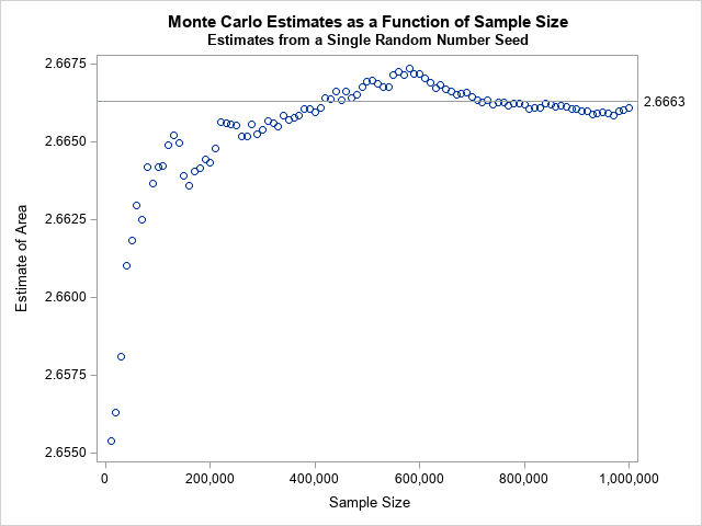
The markers in the scatter plot show the estimates for the integral when only the first k random variates are used. The horizontal line shows the exact value of the integral. For this random-number seed, the estimate stays close to the exact value when the sample size is more than 400,000. If you use a different random number seed, you will get a different graph. However, this graph is fairly typical. The Monte Carlo estimates can either overestimate or underestimate the integral.
The takeaway lesson is that the estimate converges to the exact value, but not very quickly. From general theory, we know that the standard error of the mean of n numbers is SD(Y)/sqrt(n), where SD(Y) is the standard deviation of Y for Y=g(X). That means that a 95% confidence interval for the mean has a radius 1.96*SD(Y)/sqrt(n). You can use this fact to choose a sample size so that the Monte Carlo estimate is (probably) close to the exact value of the integral. I will discuss this fact in a second article.
Summary
This article shows how to use Monte Carlo simulation to estimate a one-dimensional integral. Although Monte Carlo simulation is less accurate than other numerical integration methods, it is simple to implement and it readily generalizes to higher-dimensional integrals.

4 Comments
Rick,
Monte Carlo simulation to higher-dimensional integrals is very useful in Bayesian Analysis, due to computer is not able to perform higher-dimensional integrals . Is it right ?
People much smarter than me have developed these MCMC techniques, so I feel confident that (if done correctly) they are correct. The integrals in the MCMC analyses are (I think) always distributions, not arbitrary functions. (I guess that is mostly a matter of scaling.) In the MCMC setting, there are certain assumptions that you need to verify. The estimates from the Markov chain are not independent, so you have to check the diagnostic plots to make sure the chains are long enough and sufficiently random. In many statistical applications, you don't need the value of the integral to very many decimal places because the standard errors of the estimates are much larger than the Monte Carlo error.
The doc for the MCMC procedure has an example of estimating an integral.
Pingback: Sample size for the Monte Carlo estimate of an integral - The DO Loop
Pingback: Double integrals by using Monte Carlo methods - The DO Loop