As I discussed in a previous article, the simple block bootstrap is a way to perform a bootstrap analysis on a time series. The first step is to decompose the series into additive components: Y = Predicted + Residuals. You then choose a block length (L) that divides the total length of the series (n). Each bootstrap resample is generated by randomly choosing from among the non-overlapping n/L blocks of residuals, which are added to the predicted model.
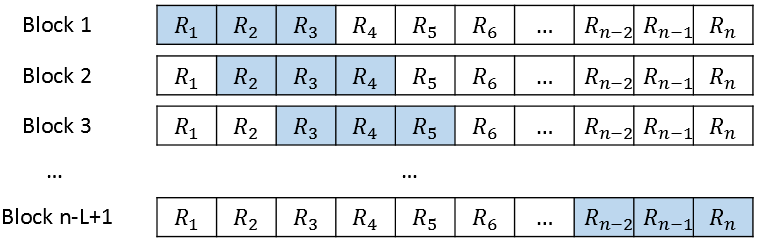
The simple block bootstrap is not often used in practice. One reason is that the total number of blocks (k=n/L) is often small. If so, the bootstrap resamples do not capture enough variation for the bootstrap method to make correct inferences. This article describes a better alternative: the moving block bootstrap. In the moving block bootstrap, every block has the same block length but the blocks overlap. The following figure illustrates the overlapping blocks when L=3. The indices 1:L define the first block of residuals, the indices 2:L+1 define the second block, and so forth until the last block, which contains the residuals n-L+1:n.
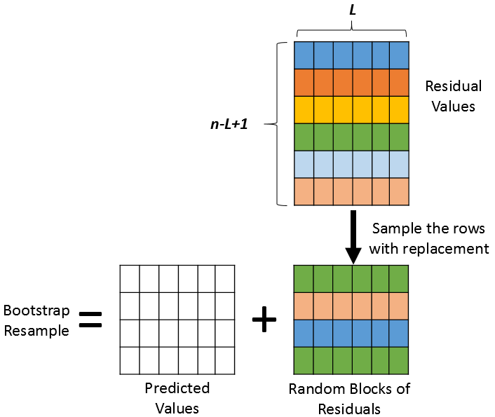
To form a bootstrap resample, you randomly choose k=n/L blocks (with replacement) and concatenate them. You then add these residuals to the predicted values to create a "new" time series. Repeat the process many times and you have constructed a batch of bootstrap resamples. The process of forming one bootstrap sample is illustrated in the following figure. In the figure, the time series has been reshaped into a k x L matrix, where each row is a block.
The moving block bootstrap in SAS
To demonstrate the moving block bootstrap in SAS, let's use the same data that I analyzed in the previous article about the simple block bootstrap. The previous article extracted 132 observations from the Sashelp.Air data set and used PROC AUTOREG to form an additive model Predicted + Residuals. The OutReg data set contains three variables of interest: Time, Pred, and Resid.
As before, I will choose the block size to be L=12. The following SAS/IML program reads the data and defines a matrix (R) such that the i_th row contains the residuals with indices i:i+L-1. In total, the matrix R has n-L+1 rows.
/* MOVING BLOCK BOOTSTRAP */ %let L = 12; proc iml; call randseed(12345); use OutReg; read all var {'Time' 'Pred' 'Resid'}; close; /* Restriction for Simple Block Bootstrap: The length of the series (n) must be divisible by the number of blocks (k) so that all blocks have the same length (L) */ n = nrow(Pred); /* length of series */ L = &L; /* length of each block */ k = n / L; /* number of random blocks to use */ if k ^= int(k) then ABORT "The series length is not divisible by the block length"; /* Trick: Reshape data into k x L matrix. Each row is block of length L */ P = shape(Pred, k, L); /* there are k rows for Pred */ J = n - L + 1; /* total number of overlapping blocks to choose from */ R = j(J, L, .); /* there are n-L+1 blocks of residuals */ Resid = rowvec(Resid); /* make Resid into row vector so we don't need to transpose each row */ do i = 1 to J; R[i,] = Resid[ , i:i+L-1]; /* fill each row with a block of residuals */ end; |
With this setup, the formation of bootstrap resamples is almost identical to the program in the previous article. The only difference is that the matrix R for the moving block bootstrap has more rows. Nevertheless, each resample is formed by randomly choosing k rows from R and adding them to a block of predicted values. The following statements generate B=1000 bootstrap resamples, which are written to a SAS data set (BootOut). The program writes the Time variable, the resampled series (YBoot), and an ID variable that identifies each bootstrap sample.
/* The moving block bootstrap repeats this process B times and usually writes the resamples to a SAS data set. */ B = 1000; SampleID = j(n,1,.); create BootOut var {'SampleID' 'Time' 'YBoot'}; /* create outside of loop */ do i = 1 to B; SampleId[,] = i; idx = sample(1:J, k); /* sample of size k from the set 1:J */ YBoot = P + R[idx,]; append; end; close BootOut; QUIT; |
The BootOut data set contains B=1000 bootstrap samples. The rest of the bootstrap analysis is exactly the same as in the previous article.
Summary
This article shows how to perform a moving block bootstrap on a time series in SAS. First, you need to decompose the series into additive components: Y = Predicted + Residuals. You then choose a block length (L), which must divide the total length of the series (n), and form the n-L+1 overlapping blocks of residuals. Each bootstrap resample is generated by randomly choosing blocks of residuals and adding them to the predicted model. This article uses the SAS/IML language to perform the simple block bootstrap in SAS.

2 Comments
Pingback: The simple block bootstrap for time series in SAS - The DO Loop
Pingback: Top 10 posts from The DO Loop in 2021 - The DO Loop