A previous article shows how to use a recursive formula to compute exact probabilities for the Poisson-binomial distribution. The recursive formula is an O(N2) computation, where N is the number of parameters for the Poisson-binomial (PB) distribution. If you have a distribution that has hundreds (or even thousands) of parameters, it might be more efficient to use a different method to approximate the PDF, CDF, and quantiles for the Poisson-binomial distribution. A fast method that is easy to implement is the Refined Normal Approximation (RNA) method, which is presented in Hong (2013, Eqn 14, p. 9-10; attributed to Volkova, 1996). This article discusses the RNA method, when to use it, and a program that implements the method in SAS.
See this introductory article for an overview of the Poisson-binomial distribution.
The normal approximation to the Poisson-binomial distribution
Before talking about the normal approximation, let's plot the exact PDF for a Poisson-binomial distribution that has 500 parameters, each a (random) value between 0 and 1. The PDF is computed by using the recursive-formula method from my previous article. Although the Poisson-binomial distribution a discrete distribution, the PDF is shown by using a series plot.
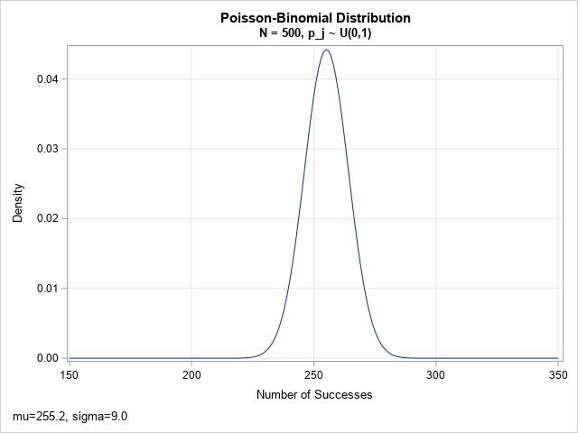
The PDF looks to be approximately normally distributed. It turns out that this is often the case when the number of parameters is large. The mean and the standard deviation of the normal approximation are easy to compute in terms of the parameters. Let p = {p1, p2, ..., pN} be the parameters for the Poisson-binomial distribution. The mean (μ), standard deviation (σ), and skewness (γ) of the distribution are given by
- μ = sum(p)
- σ = sqrt(sum(p # (1-p))), where # is the elementwise multiplication operator
- γ = sum(p # (1-p) # (1-2p)) / σ3
When N is large, the Poisson-binomial distribution is approximated by a normal distribution with mean μ and standard deviation σ. (This property also holds for the Poisson and the binomial distributions.) The PB distribution might not be symmetric, but the so-called refined normal approximation corrects for skewness in the PB distribution.
Let CDF(k; p) be the Poisson-binomial CDF. That is, CDF(k; p) is the probability of k or fewer successes among the N independent Bernoulli trials, where the probability of success for the j_th trial is p[j]. Then the refined normal approximation (RNA) is
CDF(k; p) ≈ G((k + 0.5 - μ)/σ), for k = 0, 1, ..., N
where G(x) = Φ(x) + γ (1 – x2) φ(x) / 6. Here Φ and φ are the CDF and PDF, respectively, of the standard normal distribution.
Hong (2013) presents a table (Table 2, p. 15) that shows that the refined normal approximation to the CDF is very close to the exact CDF when N ≥ 500. However, he does not mention that the mean cannot be too small or too large. As a rule of thumb, the interval [μ – 5 σ, μ + 5 σ] should be completely inside the interval [0, N]. In practical terms, you should not use the RNA when Σj pj is close to 0 or N. That is, don't use it when almost all the Bernoulli trials have very small or very large probabilities of success.
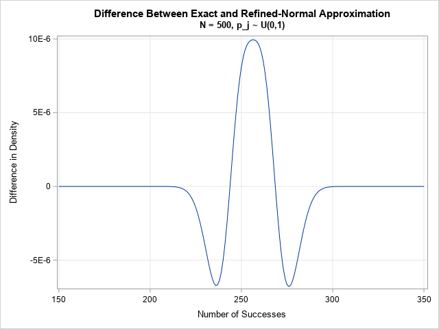
Although the computation is given for the CDF, the PDF is easier to visualize and understand. The previous graph shows the exact PDF for N=500 parameters, where each p[j]is randomly sampled from the uniform distribution on (0,1). The mean of the distribution is 255.2; the standard deviation is 9.0. For this set of parameters, the maximum difference between the EXACT distribution and the refined normal approximation is 1E-5. You can plot the difference between the exact and RNA distributions. The following plot shows that the agreement is very good. Notice that the vertical scale for the difference is tiny! The approximation is only slightly different from the approximation.
The refined normal approximation in SAS
It is straightforward to use the refined normal approximation to approximate the CDF of the Poisson-binomial distribution in SAS:
- Compute the μ, σ, and γ moments from the vector of parameters, p.
- Evaluate the refined normal approximation for each value of k.
- Because the G function is not always in the interval [0,1], use a "trap and map" technique to force extreme values into the [0,1] interval.
If you know the CDF of a discrete distribution, you can compute the difference between consecutive values to obtain the PDF. Similarly, you can use the definition of quantiles to obtain the quantile function from the PDF.
You can download the SAS program that approximates the Poisson-binomial distribution. The program, which is implemented in the SAS/IML matrix language, generates all results and graphs in this article.
Improvements in speed
The RNA algorithm is a direct method that is much faster than the recursive formula:
- For N=500, my computer computes the exact PDF in about 0.16 seconds, whereas the RNA algorithm only requires 2E-4 seconds. In other words, the RNA algorithm is about 800 times faster.
- For N=1000, the exact PDF takes about 0.6 seconds, whereas the RNA algorithm only require 3.4E-4 seconds. This is about 2000 times faster.
The RNA algorithm has a second advantage: you can directly evaluate the CDF (and PDF) functions at specific values of k. In contrast, the recursive formula, by definition, computes the distribution's value at k=j by evaluating all the previous values: k=0, 1, 2, ..., j.
Summary
In summary, when the Poisson-binomial distribution has many parameters, you can approximate the CDF and PDF by using a refined normal approximation. The normal approximation is very good when N ≥ 500 and the mean of the distribution is sufficiently far away from the values 0 and N. When those conditions are met, the RNA is a good approximation to the PB distribution. Not only is the RNA algorithm fast, but you can use it to directly compute the distribution at any value of k without computing all the earlier values.
