I recently showed how to use simulation to estimate the power of a statistical hypothesis test. The example (a two-sample t test for the difference of means) is a simple SAS/IML module that is very fast. Fast is good because often you want to perform a sequence of simulations over a range of parameter values to construct a power curve. If you need to examine 100 sets of parameter values, you would expect the full computation to take about 100 times longer than one simulation.

But that calculation applies only when you run the simulations sequentially. If you run the simulations in parallel, you can complete the simulation study much faster. For example, if you have access to a machine or cluster of machines that can run 32 threads, then each thread needs to run only a few simulations. You can perform custom parallel computations by using the iml action in SAS Viya. The iml action is supported in SAS Viya 3.5.

This article shows how to distribute computations by using the PARTASKS function in the iml action. (PARTASKS stands for PARallel TASKS.) If you are not familiar with the iml action or with parallel processing, see my previous example that uses the PARTASKS function.

Use simulation to estimate a power curve

I previously showed how to use simulation to estimate the power of a statistical test. In that article, I simulated data from N(15,5) and N(16,5) distributions. Because the t test is invariant under centering and scaling operations, this study is mathematically equivalent to simulating from the N(0,1) and N(0.2,1) distributions. (Subtract 15 and divide by 5.)

Recall that the power of a statistical hypothesis test is the probability of rejecting the null hypothesis when the alternative hypothesis is true. This is 1 minus the probability of making a "Type 2 error." (A Type 2 error is NOT rejecting H0 when H_a is true.) The power depends on the sample sizes and the magnitude of the effect you are trying to detect. In this case, the effect is the difference between two means. You can study how the power depends on the mean difference by estimating the power for a t test between data from an N(0,1) distribution and an N(δ, 1) distribution, where δ is a parameter in the interval [0, 2]. All hypothesis tests in this article use the α=0.05 significance level. To estimate the power, we will simulate many samples and compute the proportion of times that the t test rejects the null hypothesis.

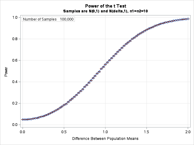
The power curve we want to estimate is shown to the right. The horizontal axis is the δ parameter, which represents the true difference between the population means. Each point on the curve is an estimate of the power of a two-sample t test for random samples of size n1 = n2 = 10. The curve indicates that when there is no difference between the means, you will conclude otherwise in 5% of random samples (because α=0.05). For larger differences, the probability of detecting the difference increases. If the difference is very large (more than 1.5 standard deviations apart), more than 90% of random samples will correctly reject the null hypothesis in the t test.

The curve is calculated at 81 values of δ, so this curve is the result of running 81 independent simulations. Each simulation uses 100,000 random samples and carries out 100,000 t tests. Although it is hard to see, the graph also shows 95% confidence intervals for power. The confidence intervals are very small because so many simulations are run.

So how long did it take to compute this power curve, which is the result of 8.1 million t tests? About 0.4 seconds by using parallel computations in the iml action.

Using the PARTASKS function to distribute tasks

Here's how you can write a program in the iml action to run 81 simulations across 32 threads. The following program uses four nodes, each with 8 threads, but you can achieve similar results by using other configurations. The main parts of the program are as follows:

• The program assumes that you have used the CAS statement in SAS to establish a CAS session that uses four worker nodes, each with at least eight CPUs. For example, the CAS statement might look something like this:
      cas sess4 host='your_host_name' casuser='your_username' port=&MPPPort nworkers=4;
  The IML program is contained between the SOURCE/ENDSOURCE statements in PROC CAS.
• The TTestH0 function implements the t test. It runs a t test on the columns of the input matrices and returns the proportion of samples that reject the null hypothesis. The TTestH0 function is explained in a previous article.
• The "task" we will distribute is the SimTTest function. (This encapsulates the "main program" in my previous article.) The SimTTest function simulates the samples, calls the TTestH0 function, and returns the number of t tests that reject the null hypothesis. The first sample is always from the N(0, 1) distribution and the second sample is from the N(δ, 1) distribution. Each call creates B samples. The input to the SimTTest function is a list that contains all parameters: a random-number seed, the sample sizes (n1 and n2), the number of samples (B), and the value of the parameter (delta).
• The main program first sets up a list of arguments for each task. The i_th item in the list is the argument to the i_th task. For this computation, all arguments are the same (a list of parameters) except that the i_th argument includes the parameter value delta[i], where delta is a vector of parameter values in the interval [0, 2].
• The call to the PARTASKS function is
       RL = ParTasks('SimTTest', ArgList, {2, 0});
  where the first parameter is the task (or list of tasks), the second parameter is the list of arguments to the tasks, and the third parameter specifies how to distribute the computations. The documentation of the PARTASKS function provides the full details.
• After the PARTASKS function returns, the program processes the results. For each value of the parameter, δ, the main statistic is the proportion of t tests (p) that reject the null hypothesis. The program also computes a 95% (Wald) confidence interval for the binomial proportion. These statistics are written to a CAS table called 'PowerCurve' by using the MatrixWriteToCAS subroutine.

/* Power curve computation: delta = 0 to 2 by 0.025 */
proc cas;
session sess4;                         /* use session with four workers     */
loadactionset 'iml';                   /* load the iml action set           */
source TTestPower;
 
/* Helper function: Compute t test for each column of X and Y.
   X is (n1 x m) matrix and Y is (n2 x m) matrix.
   Return the number of columns for which t test rejects H0 */
start TTestH0(x, y);
   n1 = nrow(X);     n2 = nrow(Y);     /* sample sizes                      */
   meanX = mean(x);  varX = var(x);    /* mean & var of each sample         */
   meanY = mean(y);  varY = var(y);
   poolStd = sqrt( ((n1-1)*varX + (n2-1)*varY) / (n1+n2-2) );
 
   /* Compute t statistic and indicator var for tests that reject H0 */
   t = (meanX - meanY) / (poolStd*sqrt(1/n1 + 1/n2));
   t_crit =  quantile('t', 1-0.05/2, n1+n2-2);       /* alpha = 0.05        */
   RejectH0 = (abs(t) > t_crit);                     /* 0 or 1              */
   return  RejectH0;                                 /* binary vector       */
finish;
 
/* Simulate two groups; Count how many reject H0: delta=0 */
start SimTTest(L);                     /* define the mapper                 */
   call randseed(L$'seed');            /* each thread uses different stream */
   x = j(L$'n1', L$'B');               /* allocate space for Group 1        */
   y = j(L$'n2', L$'B');               /* allocate space for Group 2        */
   call randgen(x, 'Normal', 0,         1);   /* X ~ N(0,1)                 */
   call randgen(y, 'Normal', L$'delta', 1);   /* Y ~ N(delta,1)             */
   return sum(TTestH0(x, y));          /* count how many reject H0          */
finish;
 
/* ----- Main Program ----- */
numSamples = 1e5;
L = [#'delta' = .,   #'n1' = 10,  #'n2' = 10,
     #'seed'  = 321, #'B'  = numSamples];
 
/* Create list of arguments. Each arg gets different value of delta */
delta = T( do(0, 2, 0.025) );
ArgList = ListCreate(nrow(delta));
do i = 1 to nrow(delta);
   L$'delta' = delta[i];
   call ListSetItem(ArgList, i, L);
end;
 
RL = ParTasks('SimTTest', ArgList, {2, 0});  /* assign nodes before threads */
 
/* Summarize results and write to CAS table for graphing */
varNames = {'Delta' 'ProbEst' 'LCL' 'UCL'};  /* names of result vars        */
Result = j(nrow(delta), 4, .);
zCrit = quantile('Normal', 1-0.05/2);  /* zCrit = 1.96                      */
do i = 1 to nrow(delta);               /* for each task                     */
   p = RL$i / numSamples;              /* get proportion that reject H0     */
   SE = sqrt(p*(1-p) / L$'B');         /* std err for binomial proportion   */
   LCL = p - zCrit*SE;                 /* 95% CI                            */
   UCL = p + zCrit*SE;
   Result[i,] = delta[i] || p || LCL || UCL;
end;
 
call MatrixWriteToCas(Result, '', 'PowerCurve', varNames);
endsource;
iml / code=TTestPower nthreads=8;
quit;

You can pull the 81 statistics back to a SAS data set and use PROC SGPLOT to plot the results. You can download the complete program that generates the statistics and graphs the power curve.

Notice that there are 81 tasks but only 32 threads. That is not a problem. The PARTASKS tries to distribute the workload as evenly as possible. In this example, 17 threads are assigned three tasks and 15 threads are assigned two tasks. If T is the time required to perform one power estimate, the total time to compute the power curve will be approximately 3T, plus "overhead costs" such as the time required to set up the problem, distribute the parameters to each task, and aggregate the results. You can minimize the overhead costs by passing only small amounts of data across nodes.

Summary

In summary, if you have a series of independent tasks in IML, you can use the PARTASKS function to distribute tasks to available threads. The speedup can be dramatic; it depends on the time required for the thread that performs the most work.

This article shows an example of using the PARTASKS function in the iml action, which is available in SAS Viya 3.5. The example shows how to distribute a sequence of computations among k threads that run concurrently and independently. In this example, k=32. Because the tasks are essentially identical, each thread computes 2/32 or 3/32 of the total work. The results from each task are returned in a list, where they can be further processed by the main program.

For more information and examples, see Wicklin and Banadaki (2020), "Write Custom Parallel Programs by Using the iml Action," which is the basis for these blog posts. Another source is the SAS IML Programming Guide, which includes documentation and examples for the iml action.